Your R workspace
Run your own code, and read the fixed code and output
R runs inside this page. Nothing is installed, and nothing you open or write leaves your browser. Start with the panel below; the sections after it explain the buttons, the data and the fixed results.
Run and save your code
First time here
- Wait for the line above Your R code to say that R is ready. R starts by itself when you open the page, which takes a few seconds.
- Read the starting code in the Your R code box. It makes five scores, then asks for their mean and their standard deviation.
- Click Run All. The answers appear under Most recent workspace output.
- Replace the starting code with your own, or click Open a CSV to bring in a data file, and run it again.
- Write what the result tells you under Your interpretation, then click Save R script and Save results and interpretation to keep both.
Open workspace for your own code or CSV
Paste the complete code for an exercise, a lab task or a homework question here, including its data-loading lines. To save edits from an example on a chapter page, copy that example's code here first.
R is starting. You can edit and save code while it loads.
Use a CSV with column names in the first row (up to 5 MB). Files stay in this browser session. For a course-supplied HSB file, open the CSV, then use hsb <- read.csv("hsb.csv").
Run Code uses the selection or current complete command. Run All uses the whole script. Clear R objects resets the analysis while keeping your code and imported files.
Your results will appear here.
What else is on this site
Use the workspace for a complete script, and read the fixed code and output for every example on the two chapter pages. For command explanations and short demonstrations, open Chapter 3 or Chapter 4. The data sources page lists every data file the site uses, with its columns and its reuse terms; the public CSVs are available at data/ paths. Open a private course CSV with Open a CSV, then run its supplied import and coding commands. The file stays in this browser session.
Save your code and results before leaving: each page has its own R session, and objects do not travel between pages.
Every example on this site uses base R with the standard stats and graphics commands; no package is loaded or installed. Programming examples use short, meaningful names such as group, score and id; when records are changed, d0 holds the starting data and dat the working copy. Calculate at full precision and report statistical results rounded once to four decimal places, with trailing zeros dropped (3.1, not 3.1000); rounded inputs or different software rounding can change the last digits. Native R output can show a different number of digits, and counts remain whole numbers.
How to run code
Run a complete example. Click Run All to run the whole code block or workspace script, including its data-loading commands.
Try commands one by one. Click inside a code box and place the cursor on the first command. Press Ctrl+Enter on Windows/Linux or Command+Return on macOS, or click Run Code. This runs the current complete command and advances the cursor. Select several commands first to run just that selection. Enter/Return alone adds a new line.
Objects remain available for later commands in the same code box. An assignment such as dat <- d0 usually prints nothing; run head(dat) to inspect the result. A command spanning several lines, such as a model or plot call with several arguments, runs together. When selecting text, include the entire command; an incomplete selection produces an R error. After changing data, rerun every calculation that uses them. Start Over restores a chapter block’s original code and clears that block’s objects.
Use desktop RStudio. Put the complete code in an R script. With the cursor on a command, Ctrl+Enter on Windows/Linux or Command+Return on macOS runs the current line or selected code. Select the whole command when it spans several lines. The RStudio shortcut reference gives further details. In the R console, type a complete command and press Enter/Return. Run the data-loading commands before commands that use them.
If R shows an error. An error stops the command. It damages nothing: your code, your objects and your imported file are all still there. Read the last line of the message first, because that line usually names the problem. Five messages come up again and again.
- R says
unexpected numeric constantorunexpected symbol. Two things sit side by side with nothing between them, usually a missing comma:c(50 54)should bec(50, 54). Put the comma in and run the line again. - R says
unexpected ')'. There is one closing bracket too many, as inc(50, 54)). Count the brackets from the left and delete the extra one. - R says
could not find function, or does not recognise a name you are sure you typed. R matches names letter for letter, sot.tsetis nott.testandMeanis notmean. Check the spelling and the capital letters. - A
+sign appears instead of a result. The command is not finished: a quotation mark or a bracket is still open and R is waiting for the rest. Complete it, or press Esc to cancel, and run the command again. - R says
object 'dat' not found. That object does not exist yet in this session, usually because the line that creates it has not been run. Run the setup lines above it, or choose Run All, and then run the command that uses the object.
Correct the line and run it again. If a code box has drifted too far from its starting code, Start Over restores it.
Saving and reopening work
Save your R script and results before leaving. The script includes unrun edits; the results file pairs the latest output with its code and the earlier executed commands. For a reproducible submission, keep all setup in the script, clear R objects, and use Run All before saving. Save plots separately. Submit through your course's usual system.
Reloading clears R objects and imported files. Reopen your CSV and saved script, then run it. On desktop R, use the folder containing your script and CSV as the working directory; built-in examples using data/... need that subfolder. For a stalled calculation, save your code and reload.
Fixed code and output
Open an example to read its starting code and saved result, even when the browser runtime is unavailable. These results describe the original data and settings; edits in a live cell or in the workspace do not change them.
The first example matches the workspace’s starting code: c() joins the scores, mean() gives their average, and sd() gives their sample standard deviation. You can also run it in desktop R. The mean is 16.4 and the sample SD is 3.0496.
scores <- c(12, 15, 17, 18, 20)
mean(scores)
[1] 16.4sd(scores)[1] 3.04959Chapter 3
These examples match the Chapter 3 page, in its order.
Normal areas, z scores and cutoffs
score <- 60
mu <- 50
sigma_known <- 5
z <- (score - mu) / sigma_known
c(z = z, lower_area = pnorm(z), upper_area = pnorm(z, lower.tail = FALSE))
z lower_area upper_area
2.00000000 0.97724987 0.02275013 pnorm(c(1, 2, 3)) - pnorm(-c(1, 2, 3))[1] 0.6826895 0.9544997 0.9973002qnorm(c(.025, .975))[1] -1.959964 1.959964A Normal model against the 395 final grades
dat <- read.csv("data/chapter_03_uci_groups.csv")
grade <- dat$final_grade
grade_mean <- mean(grade)
grade_sd <- sd(grade)
k <- 1:3
observed <- numeric(3)
for (j in k) {
  observed[j] <- mean(abs(grade - grade_mean) <= j * grade_sd)
}
round(cbind(k, observed, model = 2 * pnorm(k) - 1), 4)
k observed model
[1,] 1 0.6987 0.6827
[2,] 2 0.9013 0.9545
[3,] 3 1.0000 0.9973model_zeros <- length(grade) * pnorm(0.5, mean = grade_mean, sd = grade_sd)
round(c(observed_zeros = sum(grade == 0),
model_at_or_below_0.5 = model_zeros), 4) observed_zeros model_at_or_below_0.5
38.0000 6.0136 without <- grade[grade > 0]
round(rbind(all = c(mean = mean(grade), median = median(grade),
sd = sd(grade), IQR = IQR(grade)),
without_zeros = c(mean(without), median(without),
sd(without), IQR(without))), 4) mean median sd IQR
all 10.4152 11 4.5814 6
without_zeros 11.5238 11 3.2278 5The Special Practice interval from supplied values
estimate <- 3.1
se <- 1.13255
critical <- 1.98027
interval <- estimate + c(-1, 1) * critical * se
format(round(interval, 4), digits = 15, scientific = FALSE, trim = TRUE)
[1] "0.8572" "5.3428"One mean: known-SD z and one-sample t
n <- 25
sample_mean <- 52
null_mean <- 50
sigma_known <- 5
sample_sd <- 5
z <- (sample_mean - null_mean) / (sigma_known / sqrt(n))
t_value <- (sample_mean - null_mean) / (sample_sd / sqrt(n))
c(z = z, z_p = 2 * pnorm(-abs(z)),
  t = t_value, df = n - 1, t_p = 2 * pt(-abs(t_value), df = n - 1))
z z_p t df t_p
2.00000000 0.04550026 2.00000000 24.00000000 0.05693985 Two sample sizes with the same difference and SD
n <- c(10, 100)
difference <- 2
sample_sd <- 5
se <- sample_sd / sqrt(n)
t_value <- difference / se
p_value <- 2 * pt(-abs(t_value), df = n - 1)
data.frame(n, SE = se, t = t_value, df = n - 1, p = p_value)
n SE t df p
1 10 1.581139 1.264911 9 0.2376725632
2 100 0.500000 4.000000 99 0.0001222515Two groups: counts, means, equal-variance and Welch tests
d0 <- read.csv("data/chapter_03_special_practice.csv")
dat <- d0
head(dat)
id group score
1 C3-001 Special Practice 17
2 C3-002 Special Practice 23
3 C3-003 Special Practice 36
4 C3-004 Special Practice 20
5 C3-005 Special Practice 28
6 C3-006 Special Practice 32table(dat$group)
Special Practice   Usual Practice
              60               60
special <- dat$score[dat$group == "Special Practice"]
usual <- dat$score[dat$group == "Usual Practice"]
c(Special = mean(special), Usual = mean(usual))Special Usual
27.1 24.0 c(Special_SD = sd(special), Usual_SD = sd(usual))Special_SD Usual_SD
5.999152 6.399152 level <- 0.95
pooled <- t.test(special, usual, var.equal = TRUE, paired = FALSE,
alternative = "two.sided", conf.level = level)
welch <- t.test(special, usual, var.equal = FALSE, paired = FALSE,
alternative = "two.sided", conf.level = level)
pooled
    Two Sample t-test

data:  special and usual
t = 2.7376, df = 118, p-value = 0.007148
alternative hypothesis: true difference in means is not equal to 0
95 percent confidence interval:
 0.8575514 5.3424486
sample estimates:
mean of x mean of y
     27.1      24.0
welch
    Welch Two Sample t-test

data:  special and usual
t = 2.7376, df = 117.51, p-value = 0.007152
alternative hypothesis: true difference in means is not equal to 0
95 percent confidence interval:
 0.8574549 5.3425451
sample estimates:
mean of x mean of y
27.1 24.0 c(difference = mean(special) - mean(usual), SE = pooled$stderr)difference SE
3.100000 1.132394 pooled$conf.int[1] 0.8575514 5.3424486
attr(,"conf.level")
[1] 0.95Re-assigning the 120 records under no effect
d0 <- read.csv("data/chapter_03_special_practice.csv")
scores <- d0$score
set.seed(12345)
reassigned <- numeric(10000)
for (b in 1:10000) {
  special_rows <- sample(120, size = 60)
  reassigned[b] <- mean(scores[special_rows]) - mean(scores[-special_rows])
}
hist(reassigned, breaks = seq(-4.25, 4.25, by = 1 / 6),
     xlab = "Special-minus-Usual difference (points)", main = "")
abline(v = c(-3.1, 3.1), lty = 2)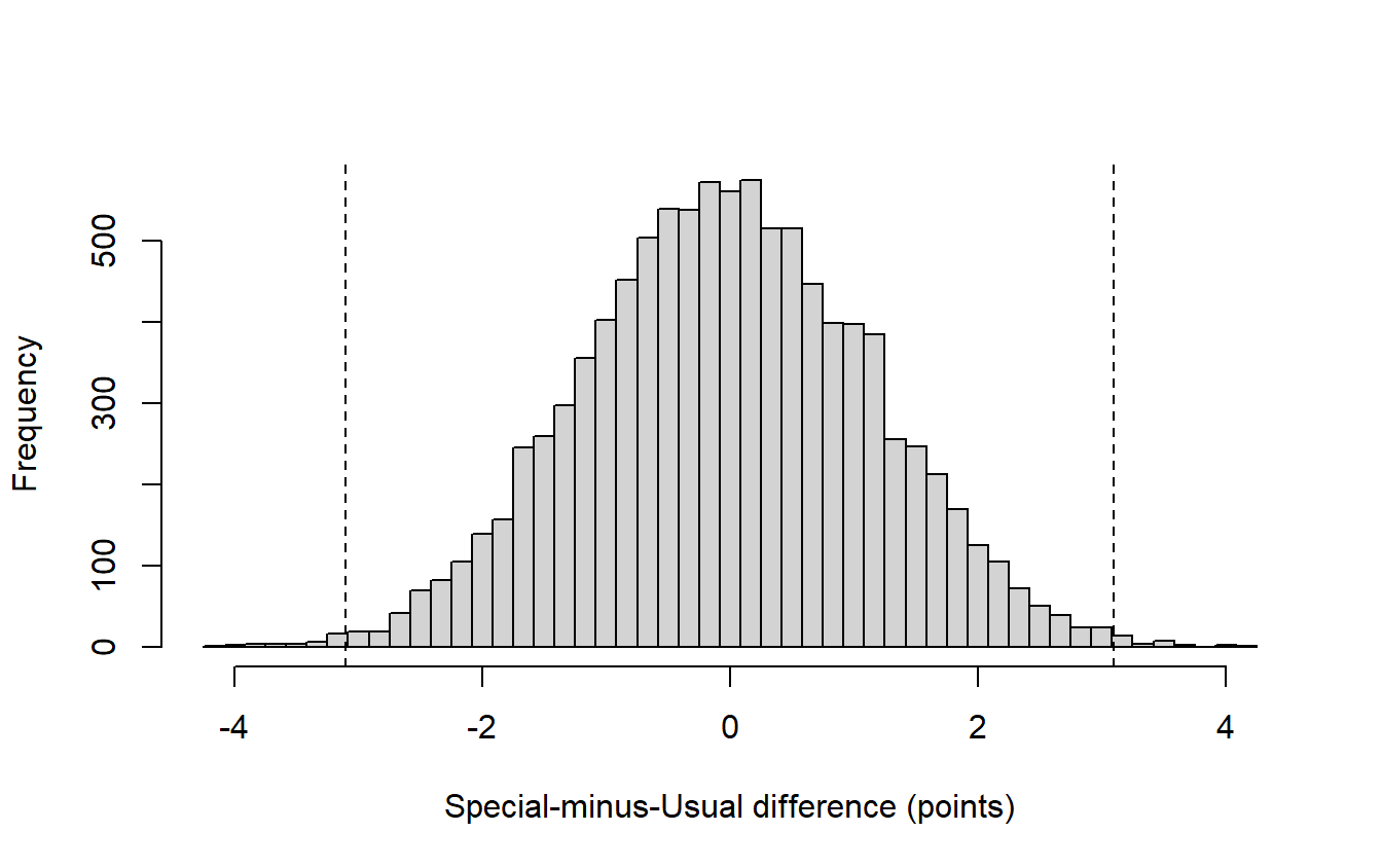
extreme <- abs(reassigned) >= 3.1 - 1e-9
c(at_least_3.1 = sum(extreme), share = mean(extreme), SD = sd(reassigned))
at_least_3.1 share SD
77.000000 0.007700 1.167111 Two programmes’ scores under the equal-variance and Welch tests
intensive <- c(18, 20, 20, 24, 29, 33, 34, 34, 38, 40)
usual <- c(16, 18, 19, 19, 20, 20, 20, 20, 20, 21, 21, 21, 22, 22, 22, 22,
           23, 23, 23, 23, 24, 24, 25, 25, 25, 25, 25, 26, 26, 26, 26, 27,
           29, 29, 29, 29, 30, 30, 32, 33)
c(mean(intensive), sd(intensive), mean(usual), sd(usual))
[1] 29 8 24 4stripchart(list(Usual = usual, Intensive = intensive), method = "stack",
pch = 16, xlab = "Assessment score (points)")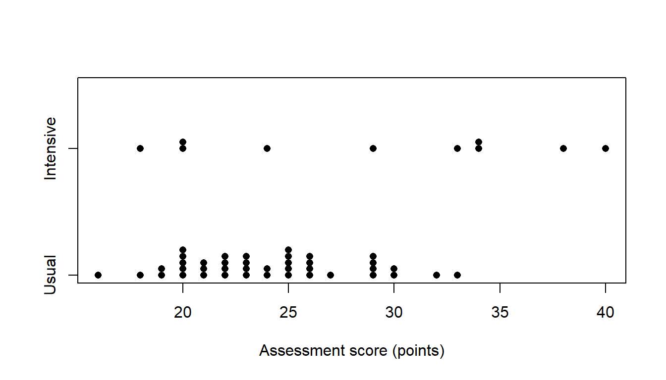
pooled <- t.test(intensive, usual, var.equal = TRUE, paired = FALSE,
                 alternative = "two.sided", conf.level = 0.95)
welch <- t.test(intensive, usual, var.equal = FALSE, paired = FALSE,
                alternative = "two.sided", conf.level = 0.95)
c(pooled_SE = pooled$stderr, welch_SE = welch$stderr,
  welch_df = unname(welch$parameter))
pooled_SE welch_SE welch_df
1.767767 2.607681 10.151006 pooled$conf.int[1] 1.445666 8.554334
attr(,"conf.level")
[1] 0.95welch$conf.int[1] -0.7985806 10.7985806
attr(,"conf.level")
[1] 0.95Unequal spreads and sizes: simulated rejection rates of the two t tests
set.seed(12345)
B <- 50000                # simulated studies
n1 <- 10                  # group sizes
n0 <- 40
s1 <- 8                   # population SDs; the population means are equal
s0 <- 4
x1 <- matrix(rnorm(B * n1, mean = 0, sd = s1), nrow = n1)  # a study per column
x0 <- matrix(rnorm(B * n0, mean = 0, sd = s0), nrow = n0)
difference <- colMeans(x1) - colMeans(x0)
v1 <- apply(x1, 2, var)
v0 <- apply(x0, 2, var)
sp2 <- ((n1 - 1) * v1 + (n0 - 1) * v0) / (n1 + n0 - 2)
se_pooled <- sqrt(sp2 * (1 / n1 + 1 / n0))
se_welch <- sqrt(v1 / n1 + v0 / n0)
nu <- (v1 / n1 + v0 / n0)^2 /
  ((v1 / n1)^2 / (n1 - 1) + (v0 / n0)^2 / (n0 - 1))
reject_pooled <- abs(difference / se_pooled) > qt(.975, df = n1 + n0 - 2)
reject_welch <- abs(difference / se_welch) > qt(.975, df = nu)
c(equal_variance = mean(reject_pooled), welch = mean(reject_welch))
equal_variance welch
0.18476 0.05070 Eight paired scores, the paired t test and the pairing ignored
before <- c(50, 54, 48, 60, 55, 58, 62, 53)
after <- c(49, 54, 49, 62, 57, 61, 66, 58)
difference <- after - before
c(n = length(difference), mean = mean(difference), SD = sd(difference))
n mean SD
8 2 2 paired_t <- t.test(after, before, paired = TRUE, mu = 0,
alternative = "two.sided", conf.level = 0.95)
paired_t
    Paired t-test

data:  after and before
t = 2.8284, df = 7, p-value = 0.02546
alternative hypothesis: true mean difference is not equal to 0
95 percent confidence interval:
 0.3279582 3.6720418
sample estimates:
mean difference
2 t.test(difference, mu = 0)
    One Sample t-test

data:  difference
t = 2.8284, df = 7, p-value = 0.02546
alternative hypothesis: true mean is not equal to 0
95 percent confidence interval:
 0.3279582 3.6720418
sample estimates:
mean of x
        2
unpaired_t <- t.test(after, before, paired = FALSE, var.equal = TRUE)
c(paired_SE = paired_t$stderr, unpaired_SE = unpaired_t$stderr) paired_SE unpaired_SE
0.7071068 2.7451256 unpaired_t$conf.int[1] -3.887709 7.887709
attr(,"conf.level")
[1] 0.95Connected paired-score plot
before <- c(50, 54, 48, 60, 55, 58, 62, 53)
after <- c(49, 54, 49, 62, 57, 61, 66, 58)
by_student <- t(cbind(before, after))
matplot(1:2, by_student, type = "b", pch = 16,
        xaxt = "n", xlab = "Measurement", ylab = "Score")
axis(1, at = 1:2, labels = c("Before", "After"))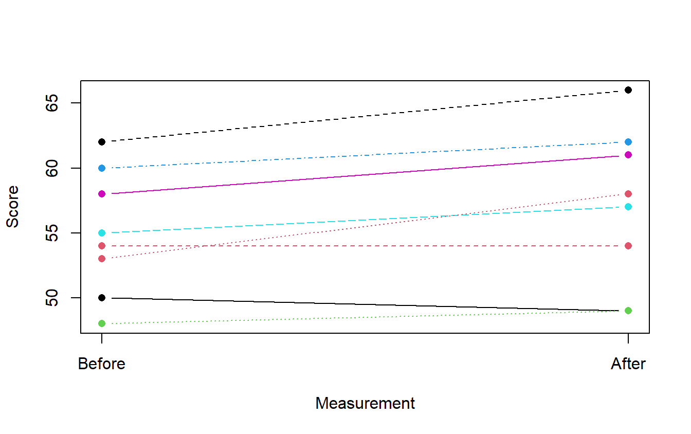
The eight after-minus-before differences
before <- c(50, 54, 48, 60, 55, 58, 62, 53)
after <- c(49, 54, 49, 62, 57, 61, 66, 58)
stripchart(after - before, method = "stack", pch = 16,
           xlab = "After minus before (points)")
abline(v = 0, lty = 2)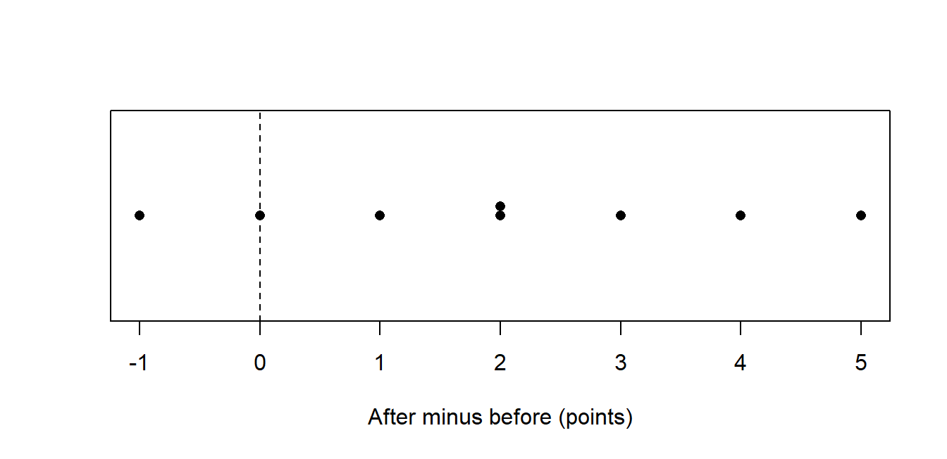
Twelve school differences and the paired t test
school_usual <- c(21, 22, 20, 23, 24, 22, 25, 24, 23, 26, 25, 22)
school_difference <- c(-2, 0, 1, 1, 2, 2, 3, 3, 4, 4, 5, 7)
school_explanatory <- school_usual + school_difference
t.test(school_explanatory, school_usual, paired = TRUE)
    Paired t-test

data:  school_explanatory and school_usual
t = 3.6187, df = 11, p-value = 0.004035
alternative hypothesis: true mean difference is not equal to 0
95 percent confidence interval:
 0.979451 4.020549
sample estimates:
mean difference
2.5 c(sum = sum(school_difference), mean = mean(school_difference),
SD = sd(school_difference),
SE_12 = sd(school_difference) / sqrt(12),
SE_480 = sd(school_difference) / sqrt(480)) sum mean SD SE_12 SE_480
30.0000000 2.5000000 2.3931721 0.6908493 0.1092329 Covariance, correlation and a unit change
x <- c(50, 54, 48, 60, 55, 58, 62, 53)
y <- c(49, 54, 49, 62, 57, 61, 66, 58)
c(covariance = cov(x, y), correlation = cor(x, y))
covariance correlation
28.1428571 0.9598913 c(covariance = cov(10 * x, y), correlation = cor(10 * x, y)) covariance correlation
281.4285714 0.9598913 cor(x, y, method = "spearman")[1] 0.9221722Histogram of the delayed-assessment scores
dat <- read.csv("data/chapter_03_special_practice.csv")
hist(dat$score, breaks = 10, main = "Special Practice study",
     xlab = "Delayed-assessment score (0-40)")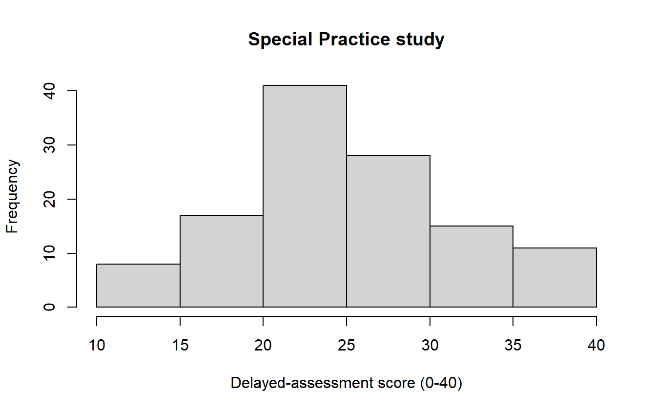
Smoothed density curve
dat <- read.csv("data/chapter_03_special_practice.csv")
plot(density(dat$score), main = "Smoothed score distribution",
     xlab = "Delayed-assessment score (0-40)")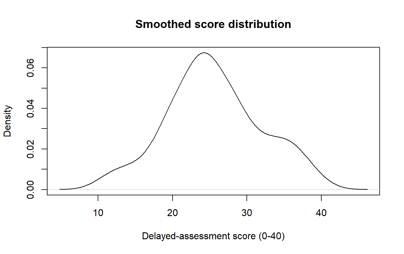
Boxplots by practice format
dat <- read.csv("data/chapter_03_special_practice.csv")
boxplot(score ~ group, data = dat, xlab = "Practice format",
        ylab = "Delayed-assessment score (0-40)")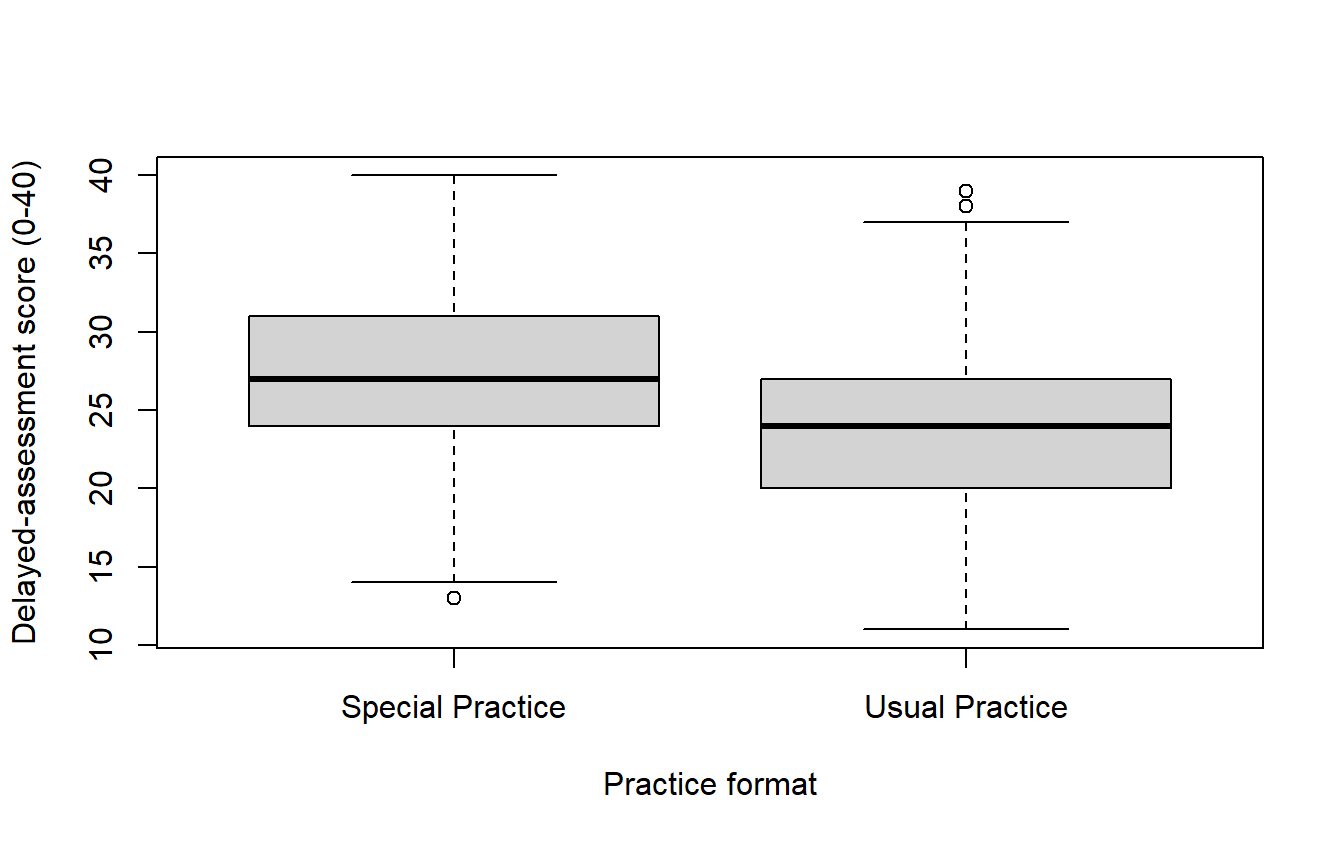
Final grades by higher-education intention
dat <- read.csv("data/chapter_03_uci_groups.csv")
boxplot(final_grade ~ higher, data = dat, horizontal = TRUE,
        xlab = "Final mathematics grade", ylab = "Intends higher education")
stripchart(final_grade ~ higher, data = dat, method = "jitter",
           pch = 16, col = "grey40", add = TRUE)
abline(v = 9.5, lty = 2)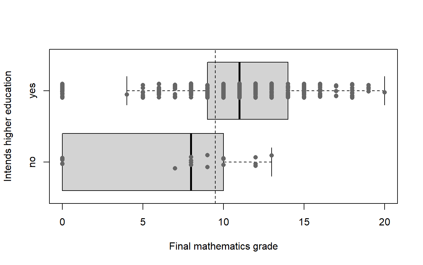
n <- table(dat$higher)
means <- tapply(dat$final_grade, dat$higher, mean)
round(cbind(n = n, mean = means,
            sd = tapply(dat$final_grade, dat$higher, sd),
            median = tapply(dat$final_grade, dat$higher, median),
            IQR = tapply(dat$final_grade, dat$higher, IQR),
            zeros = tapply(dat$final_grade == 0, dat$higher, sum)), 4)
n mean sd median IQR zeros
no 20 6.800 4.8297 8 10 6
yes 375 10.608 4.4934 11 5 32round(c(weighted = sum(n * means) / sum(n), unweighted = mean(means)), 4) weighted unweighted
10.4152 8.7040 Bar chart of the online participants
completed <- c(Completed = 32, "Not completed" = 18)
barplot(completed, ylab = "Count", main = "Online participants")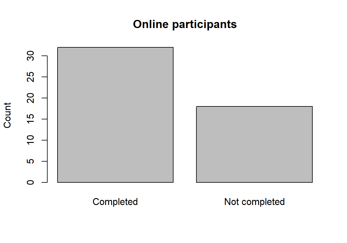
Pie chart of the same two categories
completed <- c(Completed = 32, "Not completed" = 18)
pie(completed, main = "Online completion proportions")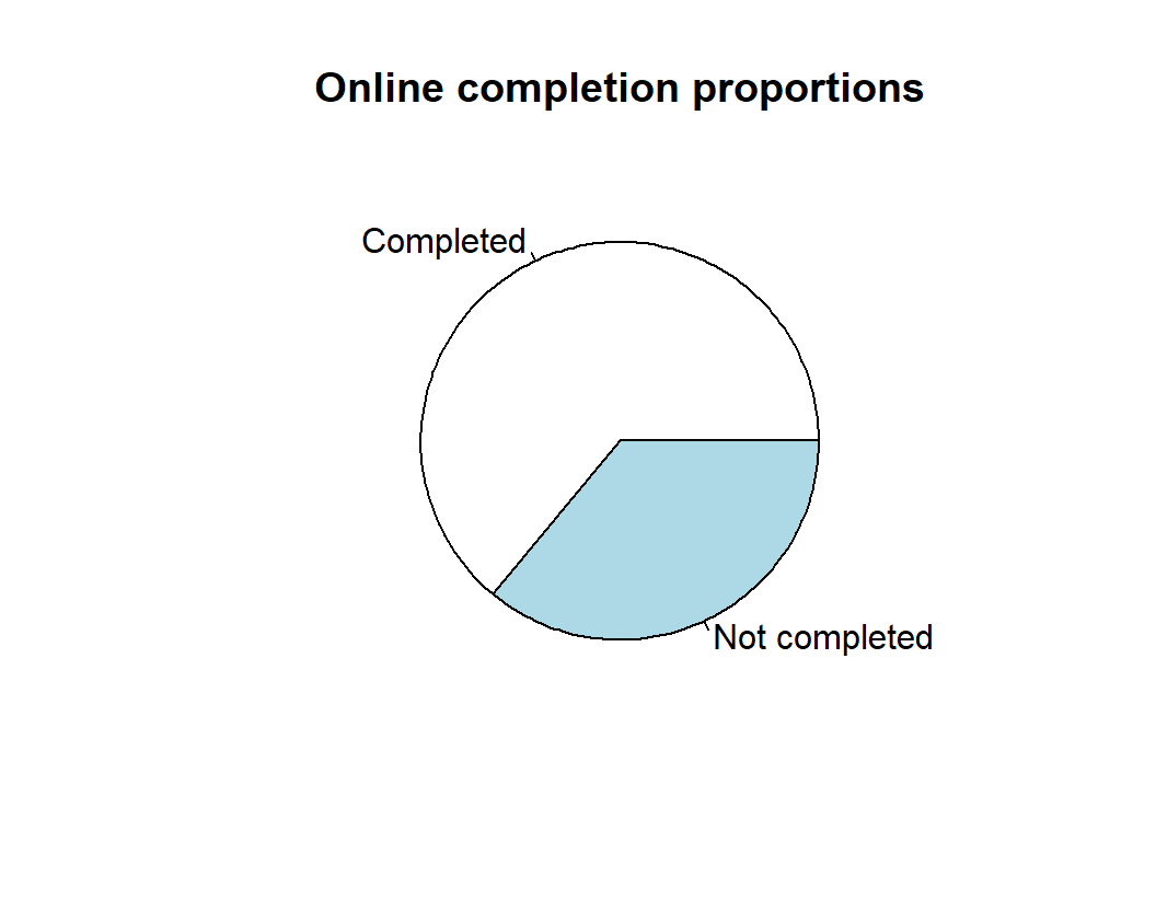
Scatterplot of before and after scores
before <- c(50, 54, 48, 60, 55, 58, 62, 53)
after <- c(49, 54, 49, 62, 57, 61, 66, 58)
plot(before, after, xlab = "Before score", ylab = "After score")
abline(a = 0, b = 1, lty = 2)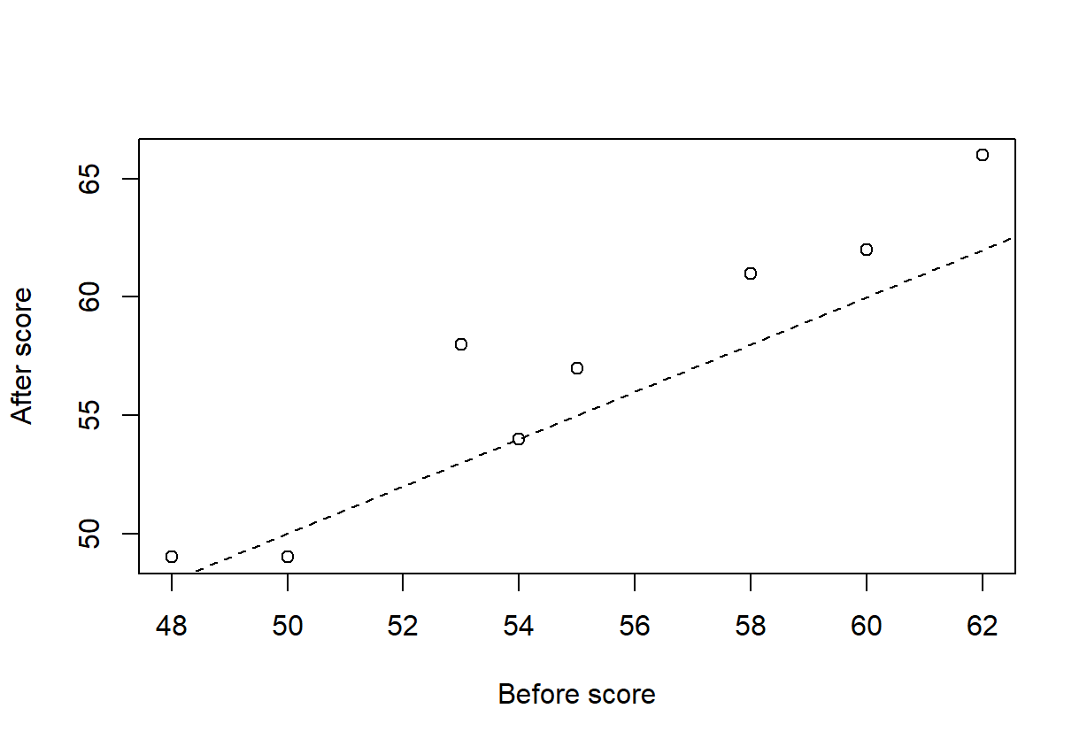
The worked two-by-two count table
counts <- matrix(c(32, 18, 18, 32), nrow = 2, byrow = TRUE,
                 dimnames = list(c("Online", "In person"),
                                 c("Completed", "Not completed")))
prop.table(counts, 1)
Completed Not completed
Online 0.64 0.36
In person 0.36 0.64pearson <- chisq.test(counts, correct = FALSE)
pearson$expected Completed Not completed
Online 25 25
In person 25 25pearson
    Pearson's Chi-squared test

data:  counts
X-squared = 7.84, df = 1, p-value = 0.00511
Exercise 7’s table and its doubled version
exercise_7 <- matrix(c(84, 36, 63, 17), nrow = 2, byrow = TRUE,
                     dimnames = list(c("Online", "In person"),
                                     c("Completed", "Not completed")))
prop.table(exercise_7, 1)
Completed Not completed
Online 0.7000 0.3000
In person 0.7875 0.2125chisq.test(exercise_7, correct = FALSE)
    Pearson's Chi-squared test

data:  exercise_7
X-squared = 1.8868, df = 1, p-value = 0.1696prop.table(2 * exercise_7, 1) Completed Not completed
Online 0.7000 0.3000
In person 0.7875 0.2125chisq.test(2 * exercise_7, correct = FALSE)
    Pearson's Chi-squared test

data:  2 * exercise_7
X-squared = 3.7736, df = 1, p-value = 0.05207
A three-way table read as two-way tables within layers
layers <- array(c(19, 15, 6, 10, 13, 3, 12, 22), dim = c(2, 2, 2),
  dimnames = list(format = c("Online", "In person"),
                  completion = c("Completed", "Not completed"),
                  prior = c("Studied before", "New to the subject")))
ftable(layers, row.vars = c("prior", "format"))
completion Completed Not completed
prior format
Studied before Online 19 6
In person 15 10
New to the subject Online 13 12
In person 3 22layers[, "Completed", ] / apply(layers, c(1, 3), sum) prior
format Studied before New to the subject
Online 0.76 0.52
In person 0.60 0.12chisq.test(layers[, , "Studied before"], correct = FALSE)
    Pearson's Chi-squared test

data:  layers[, , "Studied before"]
X-squared = 1.4706, df = 1, p-value = 0.2253chisq.test(layers[, , "New to the subject"], correct = FALSE)
    Pearson's Chi-squared test

data:  layers[, , "New to the subject"]
X-squared = 9.1912, df = 1, p-value = 0.002432
added <- apply(layers, c(1, 2), sum)
chisq.test(added, correct = FALSE)
    Pearson's Chi-squared test

data:  added
X-squared = 7.84, df = 1, p-value = 0.00511
Chapter 4
These examples match the Chapter 4 page, in its order.
The background-sound CSV, its factor order and the three groups
sound_data <- read.csv("data/background_sound.csv")
sound_data$sound <- factor(sound_data$sound,
  levels = c("Silence", "Instrumental music", "Music with lyrics"))
head(sound_data)
student sound score
1 S01 Silence 8
2 S02 Silence 9
3 S03 Silence 9
4 S04 Silence 11
5 S05 Silence 12
6 S06 Silence 13str(sound_data)'data.frame': 30 obs. of 3 variables:
$ student: chr "S01" "S02" "S03" "S04" ...
$ sound : Factor w/ 3 levels "Silence","Instrumental music",..: 1 1 1 1 1 1 1 1 1 1 ...
$ score : int 8 9 9 11 12 13 13 14 15 16 ...table(sound_data$sound)
           Silence Instrumental music  Music with lyrics
                10                 10                 10
The same 30 scores typed in
conditions <- c("Silence", "Instrumental music", "Music with lyrics")
sound_data <- data.frame(
  student = sprintf("S%02d", 1:30),
  sound = rep(conditions, each = 10),
  score = c(8, 9, 9, 11, 12, 13, 13, 14, 15, 16,
            6, 8, 8, 9, 9, 11, 11, 12, 12, 14,
            4, 5, 6, 7, 8, 8, 9, 10, 11, 12)
)
sound_data$sound <- factor(sound_data$sound, levels = conditions)
head(sound_data)
student sound score
1 S01 Silence 8
2 S02 Silence 9
3 S03 Silence 9
4 S04 Silence 11
5 S05 Silence 12
6 S06 Silence 13table(sound_data$sound)
           Silence Instrumental music  Music with lyrics
                10                 10                 10
Counts, means and SDs of the three sound conditions
sound_data <- read.csv("data/background_sound.csv")
sound_data$sound <- factor(sound_data$sound,
  levels = c("Silence", "Instrumental music", "Music with lyrics"))
table(sound_data$sound)
           Silence Instrumental music  Music with lyrics
10 10 10 aggregate(score ~ sound, data = sound_data, mean) sound score
1 Silence 12
2 Instrumental music 10
3 Music with lyrics 8tapply(sound_data$score, sound_data$sound, sd) Silence Instrumental music Music with lyrics
2.708013 2.403701 2.581989 Boxplots of the 30 scores with every student
sound_data <- read.csv("data/background_sound.csv")
sound_data$sound <- factor(sound_data$sound,
  levels = c("Silence", "Instrumental music", "Music with lyrics"))
par(mar = c(4, 10, 1, 1))
boxplot(score ~ sound, data = sound_data, horizontal = TRUE, las = 1,
        ylim = c(0, 20), col = "grey92", border = "grey40",
        xlab = "", ylab = "")
title(xlab = "Comprehension score (0-20)", line = 2.5)
set.seed(12345)
stripchart(score ~ sound, data = sound_data, method = "jitter",
           jitter = .15, pch = 16, cex = .8, add = TRUE)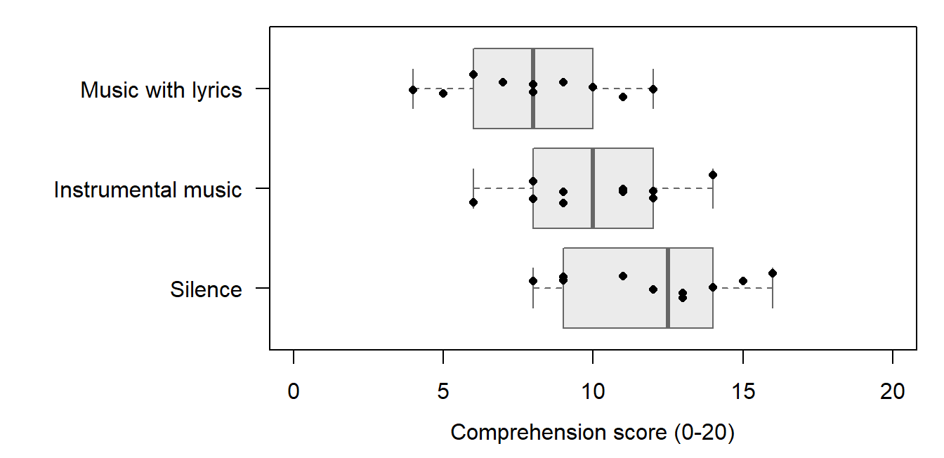
One-way ANOVA table for the background-sound study
sound_data <- read.csv("data/background_sound.csv")
sound_data$sound <- factor(sound_data$sound,
  levels = c("Silence", "Instrumental music", "Music with lyrics"))
one_way <- aov(score ~ sound, data = sound_data)
summary(one_way)
Df Sum Sq Mean Sq F value Pr(>F)
sound 2 80 40.00 6.067 0.00667 **
Residuals 27 178 6.59
---
Signif. codes: 0 '***' 0.001 '**' 0.01 '*' 0.05 '.' 0.1 ' ' 1Group variances, residual sum of squares, df, mean squares and the critical value
sound_data <- read.csv("data/background_sound.csv")
sound_data$sound <- factor(sound_data$sound,
  levels = c("Silence", "Instrumental music", "Music with lyrics"))
one_way <- aov(score ~ sound, data = sound_data)
tapply(sound_data$score, sound_data$sound, var)
Silence Instrumental music Music with lyrics
7.333333 5.777778 6.666667 SS_W <- deviance(one_way)
df_W <- df.residual(one_way)
MS_W <- SS_W / df_W
c(SS_W = SS_W, df_W = df_W, MS_W = MS_W) SS_W df_W MS_W
178.000000 27.000000 6.592593 c(MS_B = 80 / 2, F = (80 / 2) / MS_W,
p = pf((80 / 2) / MS_W, df1 = 2, df2 = df_W, lower.tail = FALSE)) MS_B F p
40.000000000 6.067415730 0.006665059 qf(.95, df1 = 2, df2 = df_W)[1] 3.354131What moves F: doubled spread, halved separation and doubled group size
sound_data <- read.csv("data/background_sound.csv")
sound_data$sound <- factor(sound_data$sound,
  levels = c("Silence", "Instrumental music", "Music with lyrics"))
group_mean <- ave(sound_data$score, sound_data$sound)
doubled <- transform(sound_data, score = group_mean + 2 * (score - group_mean))
halved <- transform(sound_data, score = score - (group_mean - 10) / 2)
anova(aov(score ~ sound, data = doubled))
Analysis of Variance Table
Response: score
Df Sum Sq Mean Sq F value Pr(>F)
sound 2 80 40.00 1.5169 0.2375
Residuals 27 712 26.37 anova(aov(score ~ sound, data = halved))Analysis of Variance Table
Response: score
Df Sum Sq Mean Sq F value Pr(>F)
sound 2 20 10.0000 1.5169 0.2375
Residuals 27 178 6.5926 group_means <- tapply(sound_data$score, sound_data$sound, mean)
group_vars <- tapply(sound_data$score, sound_data$sound, var)
SS_B_twenty <- 20 * sum((group_means - mean(group_means))^2)
SS_W_twenty <- 19 * sum(group_vars)
F_twenty <- (SS_B_twenty / 2) / (SS_W_twenty / 57)
eta_twenty <- SS_B_twenty / (SS_B_twenty + SS_W_twenty)
c(F_twenty = F_twenty,
p = pf(F_twenty, df1 = 2, df2 = 57, lower.tail = FALSE),
eta_twenty = eta_twenty) F_twenty p eta_twenty
1.213483e+01 4.068856e-05 2.986313e-01 Two declared comparisons with Silence and their Bonferroni intervals
sound_data <- read.csv("data/background_sound.csv")
sound_data$sound <- factor(sound_data$sound,
  levels = c("Silence", "Instrumental music", "Music with lyrics"))
one_way <- aov(score ~ sound, data = sound_data)
group_means <- tapply(sound_data$score, sound_data$sound, mean)
group_n <- table(sound_data$sound)
contrast_weights <- rbind(Instrumental = c(-1, 1, 0), Lyrics = c(-1, 0, 1))
estimate <- drop(contrast_weights %*% group_means)
MS_W <- deviance(one_way) / df.residual(one_way)
weight_sum <- rowSums(sweep(contrast_weights^2, 2, group_n, "/"))
SE <- sqrt(MS_W * weight_sum)
critical <- qt(1 - .05 / (2 * 2), df = df.residual(one_way))
c(critical = critical)
critical
2.373417 data.frame(estimate, SE,
lower = estimate - critical * SE,
upper = estimate + critical * SE) estimate SE lower upper
Instrumental -2 1.148268 -4.725318 0.7253181
Lyrics -4 1.148268 -6.725318 -1.2746819All three pairwise differences with Tukey
sound_data <- read.csv("data/background_sound.csv")
sound_data$sound <- factor(sound_data$sound,
  levels = c("Silence", "Instrumental music", "Music with lyrics"))
one_way <- aov(score ~ sound, data = sound_data)
TukeyHSD(one_way, which = "sound", conf.level = .95, ordered = FALSE)
Tukey multiple comparisons of means
95% family-wise confidence level
Fit: aov(formula = score ~ sound, data = sound_data)
$sound
diff lwr upr p adj
Instrumental music-Silence -2 -4.847035 0.847035 0.2084569
Music with lyrics-Silence -4 -6.847035 -1.152965 0.0046976
Music with lyrics-Instrumental music -2 -4.847035 0.847035 0.2084569One estimate under five families of comparisons
estimate <- 8 - 12
SE <- sqrt(178 / 27 * (1 / 10 + 1 / 10))
critical <- c(pointwise = qt(.975, df = 27),
  bonferroni_2 = qt(1 - .05 / (2 * 2), df = 27),
  tukey_3 = qtukey(.95, nmeans = 3, df = 27) / sqrt(2),
  bonferroni_3 = qt(1 - .05 / (2 * 3), df = 27),
  scheffe = sqrt(2 * qf(.95, df1 = 2, df2 = 27)))
lower <- estimate - critical * SE
upper <- estimate + critical * SE
round(cbind(critical, lower, upper), 4)
critical lower upper
pointwise 2.0518 -6.3561 -1.6439
bonferroni_2 2.3734 -6.7253 -1.2747
tukey_3 2.4794 -6.8470 -1.1530
bonferroni_3 2.5525 -6.9309 -1.0691
scheffe 2.5900 -6.9740 -1.0260The familywise error rate for one to ten comparisons
m <- 1:10
round(cbind(m, each_at_05 = 1 - (1 - .05)^m,
            bonferroni = 1 - (1 - .05 / m)^m), 4)
m each_at_05 bonferroni
[1,] 1 0.0500 0.0500
[2,] 2 0.0975 0.0494
[3,] 3 0.1426 0.0492
[4,] 4 0.1855 0.0491
[5,] 5 0.2262 0.0490
[6,] 6 0.2649 0.0490
[7,] 7 0.3017 0.0489
[8,] 8 0.3366 0.0489
[9,] 9 0.3698 0.0489
[10,] 10 0.4013 0.0489The feedback-by-practice CSV, its factor order and the six cells
feedback_data <- read.csv("data/feedback_practice.csv")
feedback_data$feedback <- factor(feedback_data$feedback,
  levels = c("Rereading", "Answer feedback", "Explanatory feedback"))
feedback_data$practice <- factor(feedback_data$practice,
  levels = c("Massed", "Spaced"))
head(feedback_data)
student feedback practice score
1 1 Rereading Massed 4
2 2 Rereading Massed 5
3 3 Rereading Massed 7
4 4 Rereading Massed 8
5 5 Rereading Spaced 4
6 6 Rereading Spaced 5str(feedback_data)'data.frame': 24 obs. of 4 variables:
$ student : int 1 2 3 4 5 6 7 8 9 10 ...
$ feedback: Factor w/ 3 levels "Rereading","Answer feedback",..: 1 1 1 1 1 1 1 1 2 2 ...
$ practice: Factor w/ 2 levels "Massed","Spaced": 1 1 1 1 2 2 2 2 1 1 ...
$ score : int 4 5 7 8 4 5 7 8 6 7 ...table(feedback_data$feedback, feedback_data$practice)
                       Massed Spaced
  Rereading                 4      4
  Answer feedback           4      4
  Explanatory feedback      4      4
The same 24 scores typed in
feedback_levels <- c("Rereading", "Answer feedback", "Explanatory feedback")
practice_levels <- c("Massed", "Spaced")
schedule <- rep(practice_levels, each = 4)
feedback_data <- data.frame(
  student = 1:24,
  feedback = rep(feedback_levels, each = 8),
  practice = rep(schedule, times = 3),
  score = c(4, 5, 7, 8, 4, 5, 7, 8,
            6, 7, 9, 10, 10, 11, 13, 14,
            8, 9, 11, 12, 16, 17, 19, 20)
)
feedback_data$feedback <- factor(feedback_data$feedback,
  levels = feedback_levels)
feedback_data$practice <- factor(feedback_data$practice,
  levels = practice_levels)
head(feedback_data)
student feedback practice score
1 1 Rereading Massed 4
2 2 Rereading Massed 5
3 3 Rereading Massed 7
4 4 Rereading Massed 8
5 5 Rereading Spaced 4
6 6 Rereading Spaced 5table(feedback_data$feedback, feedback_data$practice)
                       Massed Spaced
  Rereading                 4      4
  Answer feedback           4      4
  Explanatory feedback      4      4
Six cells, marginal means and the full factorial ANOVA
feedback_data <- read.csv("data/feedback_practice.csv")
feedback_data$feedback <- factor(feedback_data$feedback,
  levels = c("Rereading", "Answer feedback", "Explanatory feedback"))
feedback_data$practice <- factor(feedback_data$practice,
  levels = c("Massed", "Spaced"))
table(feedback_data$feedback, feedback_data$practice)
                       Massed Spaced
  Rereading                 4      4
  Answer feedback           4      4
  Explanatory feedback      4      4
cell_means <- tapply(feedback_data$score,
list(feedback_data$feedback, feedback_data$practice), mean)
cell_means Massed Spaced
Rereading 6 6
Answer feedback 8 12
Explanatory feedback 10 18rowMeans(cell_means) Rereading Answer feedback Explanatory feedback
6 10 14 colMeans(cell_means)Massed Spaced
8 12 full_fit <- aov(score ~ feedback * practice, data = feedback_data)
summary(full_fit) Df Sum Sq Mean Sq F value Pr(>F)
feedback 2 256 128.00 38.4 3.21e-07 ***
practice 1 96 96.00 28.8 4.23e-05 ***
feedback:practice 2 64 32.00 9.6 0.00145 **
Residuals 18 60 3.33
---
Signif. codes: 0 '***' 0.001 '**' 0.01 '*' 0.05 '.' 0.1 ' ' 1Residuals against fitted cell means
feedback_data <- read.csv("data/feedback_practice.csv")
feedback_data$feedback <- factor(feedback_data$feedback,
  levels = c("Rereading", "Answer feedback", "Explanatory feedback"))
feedback_data$practice <- factor(feedback_data$practice,
  levels = c("Massed", "Spaced"))
full_fit <- aov(score ~ feedback * practice, data = feedback_data)
par(mar = c(4, 4, 1, 1))
plot(fitted(full_fit), resid(full_fit), pch = 16,
     xlab = "Fitted cell mean", ylab = "Residual",
     xlim = c(0, 20), ylim = c(-4, 4))
abline(h = 0, lty = 2)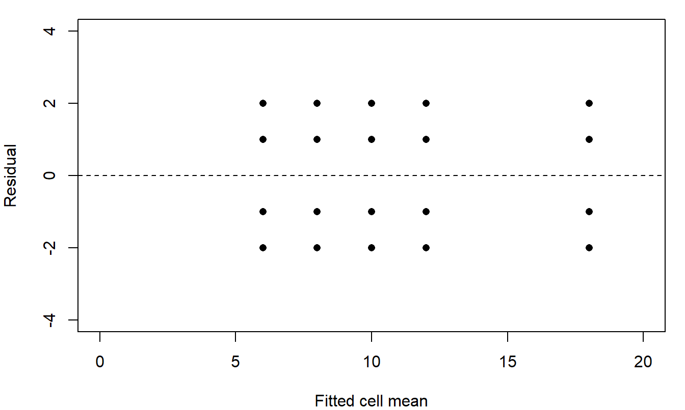
residual <- round(resid(full_fit), 4)
table(residual)
residual
-2 -1 1 2
6 6 6 6 Practice left out: the feedback-only and full-model tables
feedback_data <- read.csv("data/feedback_practice.csv")
feedback_data$feedback <- factor(feedback_data$feedback,
  levels = c("Rereading", "Answer feedback", "Explanatory feedback"))
feedback_data$practice <- factor(feedback_data$practice,
  levels = c("Massed", "Spaced"))
boxplot(score ~ feedback, data = feedback_data, ylim = c(0, 20),
  xlab = "Feedback condition", ylab = "Quiz score (0-20)")
points(as.integer(feedback_data$feedback) +
    ifelse(feedback_data$practice == "Massed", -0.1, 0.1),
  feedback_data$score,
  pch = ifelse(feedback_data$practice == "Massed", 16, 2))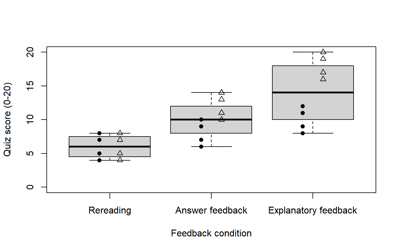
feedback_only <- aov(score ~ feedback, data = feedback_data)
full_fit <- aov(score ~ feedback * practice, data = feedback_data)
anova(feedback_only)
Analysis of Variance Table
Response: score
Df Sum Sq Mean Sq F value Pr(>F)
feedback 2 256 128.000 12.218 0.0003024 ***
Residuals 21 220 10.476
---
Signif. codes: 0 '***' 0.001 '**' 0.01 '*' 0.05 '.' 0.1 ' ' 1anova(full_fit)Analysis of Variance Table
Response: score
Df Sum Sq Mean Sq F value Pr(>F)
feedback 2 256 128.000 38.4 3.208e-07 ***
practice 1 96 96.000 28.8 4.229e-05 ***
feedback:practice 2 64 32.000 9.6 0.001454 **
Residuals 18 60 3.333
---
Signif. codes: 0 '***' 0.001 '**' 0.01 '*' 0.05 '.' 0.1 ' ' 1tapply(feedback_data$score, feedback_data$feedback, sd) Rereading Answer feedback Explanatory feedback
1.690309 2.725541 4.598136 Eta squared for the one-way and factorial fits
sound_data <- read.csv("data/background_sound.csv")
sound_data$sound <- factor(sound_data$sound,
  levels = c("Silence", "Instrumental music", "Music with lyrics"))
one_way <- aov(score ~ sound, data = sound_data)
one_SS <- anova(one_way)[["Sum Sq"]]
c(SS_B = one_SS[1], SS_W = one_SS[2], SS_T = sum(one_SS),
  eta_squared = one_SS[1] / sum(one_SS))
SS_B SS_W SS_T eta_squared
80.0000000 178.0000000 258.0000000 0.3100775 feedback_data <- read.csv("data/feedback_practice.csv")
feedback_data$feedback <- factor(feedback_data$feedback,
levels = c("Rereading", "Answer feedback", "Explanatory feedback"))
feedback_data$practice <- factor(feedback_data$practice,
levels = c("Massed", "Spaced"))
full_fit <- aov(score ~ feedback * practice, data = feedback_data)
full_table <- anova(full_fit)
full_SS <- full_table[["Sum Sq"]]
names(full_SS) <- rownames(full_table)
full_SS feedback practice feedback:practice Residuals
256 96 64 60 round(full_SS / sum(full_SS), 4) feedback practice feedback:practice Residuals
0.5378 0.2017 0.1345 0.1261 Interaction plot of the six cell means
feedback_data <- read.csv("data/feedback_practice.csv")
feedback_data$feedback <- factor(feedback_data$feedback,
  levels = c("Rereading", "Answer feedback", "Explanatory feedback"))
feedback_data$practice <- factor(feedback_data$practice,
  levels = c("Massed", "Spaced"))
par(mar = c(4, 4, 1, 1))
interaction.plot(feedback_data$practice, feedback_data$feedback,
                 feedback_data$score, type = "b",
                 pch = c(16, 1, 17), lty = 1:3,
                 xlab = "Practice schedule", ylab = "Mean quiz score",
                 trace.label = "Feedback", ylim = c(0, 20))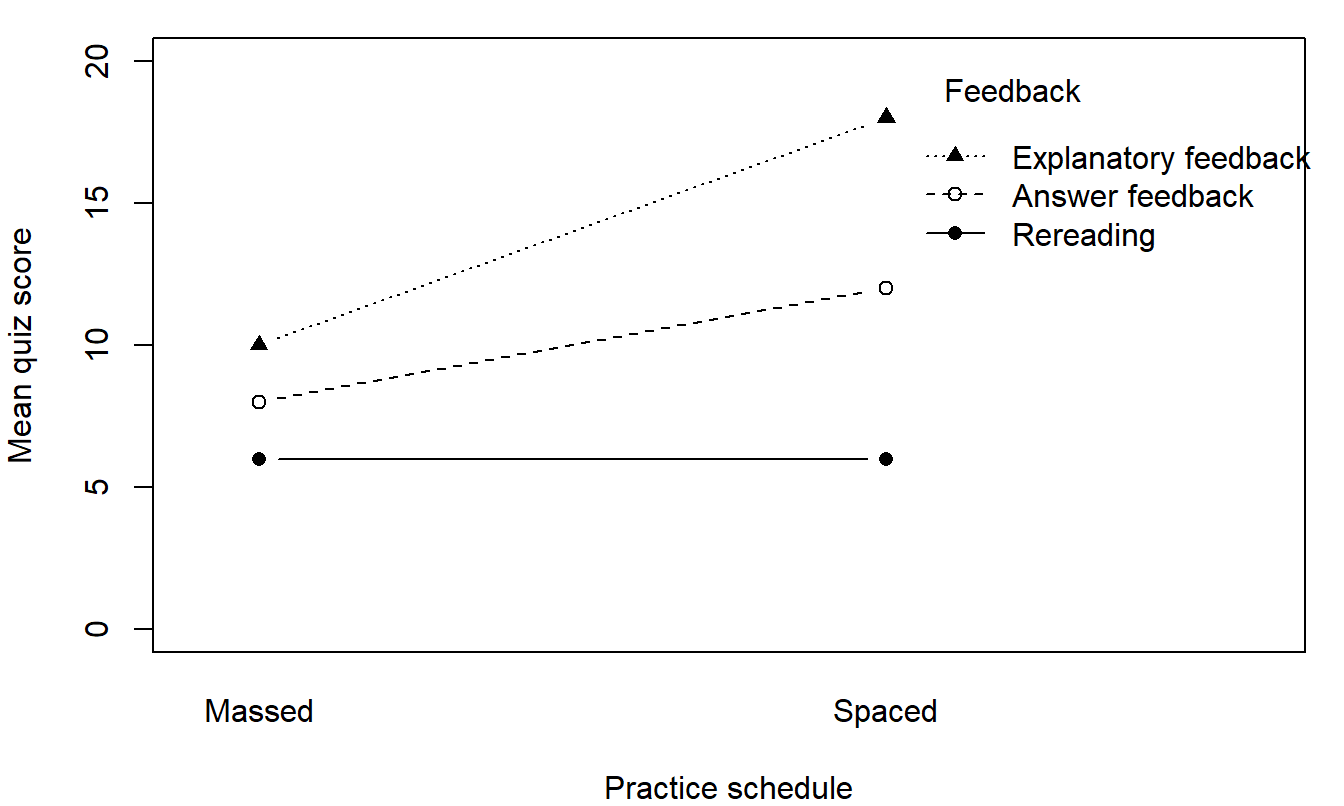
Schedule differences and the declared interval
feedback_data <- read.csv("data/feedback_practice.csv")
feedback_data$feedback <- factor(feedback_data$feedback,
  levels = c("Rereading", "Answer feedback", "Explanatory feedback"))
feedback_data$practice <- factor(feedback_data$practice,
  levels = c("Massed", "Spaced"))
full_fit <- aov(score ~ feedback * practice, data = feedback_data)
cell_means <- tapply(feedback_data$score,
  list(feedback_data$feedback, feedback_data$practice), mean)
schedule_difference <- cell_means[, "Spaced"] - cell_means[, "Massed"]
schedule_difference
Rereading Answer feedback Explanatory feedback
0 4 8 declared <- schedule_difference["Answer feedback"] -
schedule_difference["Rereading"]
error_df <- df.residual(full_fit)
MS_E <- deviance(full_fit) / error_df
declared_SE <- sqrt(MS_E * (1 / 4 + 1 / 4 + 1 / 4 + 1 / 4))
critical <- qt(.975, df = error_df)
c(estimate = unname(declared), SE = declared_SE, multiplier = critical) estimate SE multiplier
4.000000 1.825742 2.100922 interval <- unname(declared) + c(-1, 1) * critical * declared_SE
format(round(interval, 4), digits = 15, scientific = FALSE, trim = TRUE)[1] "0.1643" "7.8357"Welch’s one-way ANOVA beside the classical F
sound_data <- read.csv("data/background_sound.csv")
sound_data$sound <- factor(sound_data$sound,
  levels = c("Silence", "Instrumental music", "Music with lyrics"))
tapply(sound_data$score, sound_data$sound, sd)
Silence Instrumental music Music with lyrics
2.708013 2.403701 2.581989 classical <- oneway.test(score ~ sound, data = sound_data, var.equal = TRUE)
welch <- oneway.test(score ~ sound, data = sound_data, var.equal = FALSE)
classical
    One-way analysis of means

data:  score and sound
F = 6.0674, num df = 2, denom df = 27, p-value = 0.006665
welch
    One-way analysis of means (not assuming equal variances)

data:  score and sound
F = 5.5144, num df = 2.000, denom df = 17.956, p-value = 0.01358
Unequal spreads and sizes: simulated rejection rates of the two F tests
set.seed(12345)
B <- 50000                 # simulated studies
n <- c(10, 20, 40)         # group sizes
s <- c(8, 4, 4)            # population SDs; the population means are equal
J <- length(n)
N <- sum(n)
means <- matrix(NA, nrow = B, ncol = J)   # a study per row
vars <- matrix(NA, nrow = B, ncol = J)
for (j in 1:J) {
  # each column of x is one simulated study of group j
  x <- matrix(rnorm(B * n[j], mean = 0, sd = s[j]), nrow = n[j])
  means[, j] <- colMeans(x)
  vars[, j] <- apply(x, 2, var)
}
grand <- drop(means %*% n) / N
MS_B <- drop((means - grand)^2 %*% n) / (J - 1)
MS_W <- drop(vars %*% (n - 1)) / (N - J)
reject_classical <- MS_B / MS_W > qf(.95, df1 = J - 1, df2 = N - J)
w <- sweep(1 / vars, 2, n, "*")                   # weights n_j / s_j^2
W <- rowSums(w)
weighted_mean <- rowSums(w * means) / W
S <- drop((1 - w / W)^2 %*% (1 / (n - 1)))
F_welch <- rowSums(w * (means - weighted_mean)^2) / (J - 1) /
  (1 + 2 * (J - 2) / (J^2 - 1) * S)
nu <- (J^2 - 1) / (3 * S)
reject_welch <- F_welch > qf(.95, df1 = J - 1, df2 = nu)
c(classical = mean(reject_classical), welch = mean(reject_welch))
classical welch
0.15724 0.05106