pcfa-examples
Jinsong Chen
2022-05-15
Source:vignettes/Examples/pcfa-examples.Rmd
pcfa-examples.RmdNote: the estimation process can be time consuming depending on the computing power. You can same some time by reducing the length of the chains.
Continuous Data w/o Local Dependence:
- Load the package, obtain the data, and check the true loading pattern (qlam) and local dependence.
## LAWBL Package (version 1.5.0; 2022-05-13)
## For tutorials, see https://jinsong-chen.github.io/LAWBL/
dat <- sim18cfa0$dat
J <- ncol(dat) # no. of items
K <- 3 # no. of factors
sim18cfa0$qlam
## [,1] [,2] [,3]
## [1,] 0.7 0.0 0.0
## [2,] 0.7 0.0 0.0
## [3,] 0.7 0.0 0.0
## [4,] 0.7 0.0 0.0
## [5,] 0.7 0.3 0.0
## [6,] 0.7 0.3 0.0
## [7,] 0.0 0.7 0.0
## [8,] 0.0 0.7 0.0
## [9,] 0.0 0.7 0.0
## [10,] 0.0 0.7 0.0
## [11,] 0.0 0.7 0.3
## [12,] 0.0 0.7 0.3
## [13,] 0.0 0.0 0.7
## [14,] 0.0 0.0 0.7
## [15,] 0.0 0.0 0.7
## [16,] 0.0 0.0 0.7
## [17,] 0.3 0.0 0.7
## [18,] 0.3 0.0 0.7
sim18cfa0$LD## row col- E-step: Estimate with the PCFA-LI model (E-step) by setting LD=F and the design matrix Q. Only a few loadings need to be specified in Q (e.g., 2 per factor). Longer chain is suggested for stabler performance (burn=iter=5,000 by default).
Q<-matrix(-1,J,K); # -1 for unspecified items
Q[1:2,1]<-Q[7:8,2]<-Q[13:14,3]<-1 # 1 for specified items
Q
## [,1] [,2] [,3]
## [1,] 1 -1 -1
## [2,] 1 -1 -1
## [3,] -1 -1 -1
## [4,] -1 -1 -1
## [5,] -1 -1 -1
## [6,] -1 -1 -1
## [7,] -1 1 -1
## [8,] -1 1 -1
## [9,] -1 -1 -1
## [10,] -1 -1 -1
## [11,] -1 -1 -1
## [12,] -1 -1 -1
## [13,] -1 -1 1
## [14,] -1 -1 1
## [15,] -1 -1 -1
## [16,] -1 -1 -1
## [17,] -1 -1 -1
## [18,] -1 -1 -1## $NJK
## [1] 1000 18 3
##
## $`Miss%`
## [1] 0
##
## $`LD Allowed`
## [1] FALSE
##
## $`Burn in`
## [1] 5000
##
## $Iteration
## [1] 5000
##
## $`No. of sig lambda`
## [1] 24
##
## $Selected
## [1] TRUE TRUE TRUE
##
## $`Auto, NCONV, MCONV`
## [1] 0 0 10
##
## $EPSR
## Point est. Upper C.I.
## [1,] 1.0624 1.0667
## [2,] 1.0780 1.0824
## [3,] 1.0324 1.1183
##
## $`DIC, BIC, AIC`
## [1] 4855.375 2701.101 2333.019
##
## $Time
## user system elapsed
## 42.42 0.08 42.55
#summarize significant loadings in pattern/Q-matrix format
summary(m0, what = 'qlambda')
## 1 2 3
## I1 0.7134 0.0000 0.0000
## I2 0.7274 0.0000 0.0000
## I3 0.7343 0.0000 0.0000
## I4 0.7523 0.0000 0.0000
## I5 0.7324 0.2731 0.0000
## I6 0.7060 0.2893 0.0000
## I7 0.0000 0.7340 0.0000
## I8 0.0000 0.7310 0.0000
## I9 0.0000 0.7421 0.0000
## I10 0.0000 0.7262 0.0000
## I11 0.0000 0.7115 0.2661
## I12 0.0000 0.7021 0.2487
## I13 0.0000 0.0000 0.7028
## I14 0.0000 0.0000 0.6825
## I15 0.0000 0.0000 0.7151
## I16 0.0000 0.0000 0.7147
## I17 0.2909 0.0000 0.6870
## I18 0.2787 0.0000 0.6920
#factorial eigenvalue
summary(m0,what='eigen')
## est sd lower upper sig
## F1 3.4409 0.5717 2.5379 4.7755 1
## F2 3.4564 0.4431 2.7413 4.4195 1
## F3 3.1777 0.4515 2.3685 4.0800 1
#plotting factorial eigenvalue
plot_lawbl(m0) # trace
plot_lawbl(m0, what='density') #density
plot_lawbl(m0, what='EPSR') #EPSR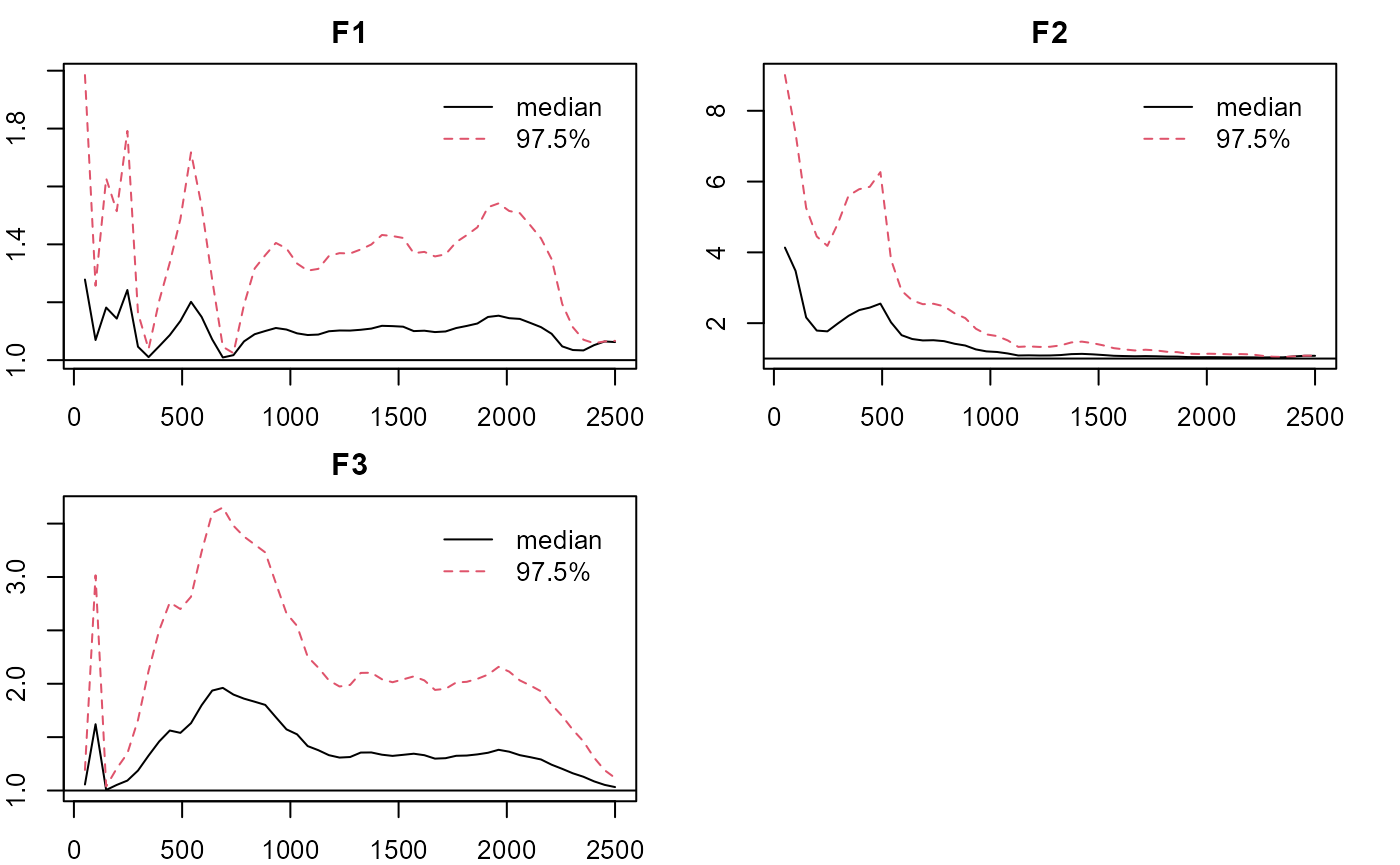
- C-step: Reconfigure the Q matrix for the C-step with one specified loading per item based on results from the E-step. Estimate with the PCFA model by setting LD=TRUE (by default). Longer chain is suggested for stabler performance. Results are very close to the E-step, since there’s no LD in the data.
Q<-matrix(-1,J,K);
tmp<-summary(m0, what="qlambda")
cind<-apply(tmp,1,which.max)
Q[cbind(c(1:J),cind)]<-1
#alternatively
#Q[1:6,1]<-Q[7:12,2]<-Q[13:18,3]<-1 # 1 for specified items

m1 <- pcfa(dat = dat, Q = Q)
summary(m1)
## $NJK
## [1] 1000 18 3
##
## $`Miss%`
## [1] 0
##
## $`LD Allowed`
## [1] TRUE
##
## $`Burn in`
## [1] 5000
##
## $Iteration
## [1] 5000
##
## $`No. of sig lambda`
## [1] 24
##
## $Selected
## [1] TRUE TRUE TRUE
##
## $`Auto, NCONV, MCONV`
## [1] 0 0 10
##
## $EPSR
## Point est. Upper C.I.
## [1,] 1.0180 1.0589
## [2,] 1.0253 1.0897
## [3,] 1.0008 1.0009
##
## $`No. of sig LD terms`
## [1] 0
##
## $`DIC, BIC, AIC`
## [1] 5323.362 4298.661 3179.693
##
## $Time
## user system elapsed
## 109.48 0.01 109.62
summary(m1, what = 'qlambda')## 1 2 3
## I1 0.6787 0.0000 0.0000
## I2 0.7055 0.0000 0.0000
## I3 0.7096 0.0000 0.0000
## I4 0.7309 0.0000 0.0000
## I5 0.7080 0.2743 0.0000
## I6 0.6785 0.2920 0.0000
## I7 0.0000 0.7332 0.0000
## I8 0.0000 0.7218 0.0000
## I9 0.0000 0.7379 0.0000
## I10 0.0000 0.7240 0.0000
## I11 0.0000 0.7099 0.2376
## I12 0.0000 0.7052 0.2253
## I13 0.0000 0.0000 0.6985
## I14 0.0000 0.0000 0.6740
## I15 0.0000 0.0000 0.7154
## I16 0.0000 0.0000 0.7082
## I17 0.2479 0.0000 0.6910
## I18 0.2345 0.0000 0.6977
summary(m1, what = 'offpsx') #summarize significant LD terms## row col est sd lower upper sig
summary(m1,what='eigen')## est sd lower upper sig
## F1 3.1446 0.2822 2.6145 3.7453 1
## F2 3.3541 0.2975 2.8197 3.9469 1
## F3 3.1052 0.2789 2.6008 3.6856 1
#plotting factorial eigenvalue
# par(mar = rep(2, 4))
plot_lawbl(m1) # trace
plot_lawbl(m1, what='density') #density
plot_lawbl(m1, what='EPSR') #EPSR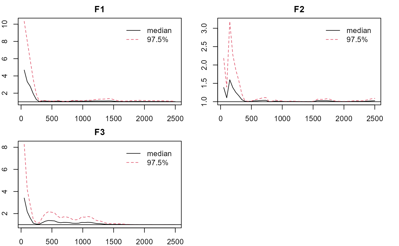
- CFA-LD: One can also configure the Q matrix for a CFA model with local dependence (i.e. without any unspecified loading) based on results from the C-step. Results are also very close.
Q<-summary(m1, what="qlambda")
Q[Q!=0]<-1
Q
## 1 2 3
## I1 1 0 0
## I2 1 0 0
## I3 1 0 0
## I4 1 0 0
## I5 1 1 0
## I6 1 1 0
## I7 0 1 0
## I8 0 1 0
## I9 0 1 0
## I10 0 1 0
## I11 0 1 1
## I12 0 1 1
## I13 0 0 1
## I14 0 0 1
## I15 0 0 1
## I16 0 0 1
## I17 1 0 1
## I18 1 0 1## $NJK
## [1] 1000 18 3
##
## $`Miss%`
## [1] 0
##
## $`LD Allowed`
## [1] TRUE
##
## $`Burn in`
## [1] 5000
##
## $Iteration
## [1] 5000
##
## $`No. of sig lambda`
## [1] 24
##
## $Selected
## [1] TRUE TRUE TRUE
##
## $`Auto, NCONV, MCONV`
## [1] 0 0 10
##
## $EPSR
## Point est. Upper C.I.
## [1,] 1.0081 1.0153
## [2,] 1.0122 1.0583
## [3,] 1.0057 1.0203
##
## $`No. of sig LD terms`
## [1] 0
##
## $`DIC, BIC, AIC`
## [1] 5122.965 3670.614 2698.878
##
## $Time
## user system elapsed
## 81.42 0.03 81.55
summary(m2, what = 'qlambda') ## 1 2 3
## I1 0.6829 0.0000 0.0000
## I2 0.6974 0.0000 0.0000
## I3 0.7117 0.0000 0.0000
## I4 0.7103 0.0000 0.0000
## I5 0.6830 0.3292 0.0000
## I6 0.6707 0.3427 0.0000
## I7 0.0000 0.7294 0.0000
## I8 0.0000 0.7251 0.0000
## I9 0.0000 0.7245 0.0000
## I10 0.0000 0.6925 0.0000
## I11 0.0000 0.6935 0.2903
## I12 0.0000 0.6907 0.2914
## I13 0.0000 0.0000 0.6747
## I14 0.0000 0.0000 0.6791
## I15 0.0000 0.0000 0.7174
## I16 0.0000 0.0000 0.6660
## I17 0.3112 0.0000 0.6787
## I18 0.2866 0.0000 0.6812
summary(m2, what = 'offpsx')## row col est sd lower upper sig
summary(m2,what='eigen')## est sd lower upper sig
## F1 3.0682 0.1615 2.7644 3.3982 1
## F2 3.2549 0.1830 2.9039 3.6055 1
## F3 2.9784 0.1751 2.6335 3.3177 1
plot_lawbl(m2) # Eigens' traces are excellent without regularization of the loadings
Continuous Data with Local Dependence:
- Obtain the data and check the true loading pattern (qlam) and local dependence.
dat <- sim18cfa1$dat
J <- ncol(dat) # no. of items
K <- 3 # no. of factors
sim18cfa1$qlam
## [,1] [,2] [,3]
## [1,] 0.7 0.0 0.0
## [2,] 0.7 0.0 0.0
## [3,] 0.7 0.0 0.0
## [4,] 0.7 0.0 0.0
## [5,] 0.7 0.3 0.0
## [6,] 0.7 0.3 0.0
## [7,] 0.0 0.7 0.0
## [8,] 0.0 0.7 0.0
## [9,] 0.0 0.7 0.0
## [10,] 0.0 0.7 0.0
## [11,] 0.0 0.7 0.3
## [12,] 0.0 0.7 0.3
## [13,] 0.0 0.0 0.7
## [14,] 0.0 0.0 0.7
## [15,] 0.0 0.0 0.7
## [16,] 0.0 0.0 0.7
## [17,] 0.3 0.0 0.7
## [18,] 0.3 0.0 0.7
sim18cfa1$LD # effect size = .3## row col
## [1,] 14 1
## [2,] 7 2
## [3,] 4 3
## [4,] 13 8
## [5,] 10 9
## [6,] 16 15- E-step: Estimate with the PCFA-LI model (E-step) by setting LD=FALSE and the design matrix Q. Only a few loadings need to be specified in Q (e.g., 2 per factor). Some loading estimates are biased due to ignoring the LD. So do the eigenvalues.
Q<-matrix(-1,J,K); # -1 for unspecified items
Q[1:2,1]<-Q[7:8,2]<-Q[13:14,3]<-1 # 1 for specified items
Q
## [,1] [,2] [,3]
## [1,] 1 -1 -1
## [2,] 1 -1 -1
## [3,] -1 -1 -1
## [4,] -1 -1 -1
## [5,] -1 -1 -1
## [6,] -1 -1 -1
## [7,] -1 1 -1
## [8,] -1 1 -1
## [9,] -1 -1 -1
## [10,] -1 -1 -1
## [11,] -1 -1 -1
## [12,] -1 -1 -1
## [13,] -1 -1 1
## [14,] -1 -1 1
## [15,] -1 -1 -1
## [16,] -1 -1 -1
## [17,] -1 -1 -1
## [18,] -1 -1 -1## $NJK
## [1] 1000 18 3
##
## $`Miss%`
## [1] 0
##
## $`LD Allowed`
## [1] FALSE
##
## $`Burn in`
## [1] 5000
##
## $Iteration
## [1] 5000
##
## $`No. of sig lambda`
## [1] 22
##
## $Selected
## [1] TRUE TRUE TRUE
##
## $`Auto, NCONV, MCONV`
## [1] 0 0 10
##
## $EPSR
## Point est. Upper C.I.
## [1,] 1.0268 1.1202
## [2,] 1.3077 2.1823
## [3,] 1.0682 1.2584
##
## $`DIC, BIC, AIC`
## [1] 3729.068 2180.126 1812.044
##
## $Time
## user system elapsed
## 36.11 0.05 36.19
summary(m0, what = 'qlambda')## 1 2 3
## I1 0.6508 0.0000 0.0000
## I2 0.6538 0.0000 0.0000
## I3 0.8787 0.0000 0.0000
## I4 0.8822 0.0000 0.0000
## I5 0.6997 0.2283 0.0000
## I6 0.6745 0.2398 0.0000
## I7 0.0000 0.7103 0.0000
## I8 0.0000 0.6613 0.0000
## I9 0.0000 0.9186 0.0000
## I10 0.0000 0.9091 0.0000
## I11 0.0000 0.6889 0.0000
## I12 0.0000 0.7078 0.0000
## I13 0.0000 0.0000 0.6723
## I14 0.0000 0.0000 0.6606
## I15 0.0000 0.0000 0.7828
## I16 0.0000 0.0000 0.7876
## I17 0.3045 0.0000 0.6567
## I18 0.2978 0.0000 0.6622
summary(m0,what='eigen')## est sd lower upper sig
## F1 3.6387 0.4013 2.8974 4.4469 1
## F2 3.7860 0.4673 2.9911 4.6466 1
## F3 3.3188 0.4206 2.5796 4.2597 1
plot_lawbl(m0) # trace
plot_lawbl(m0, what='EPSR') #EPSR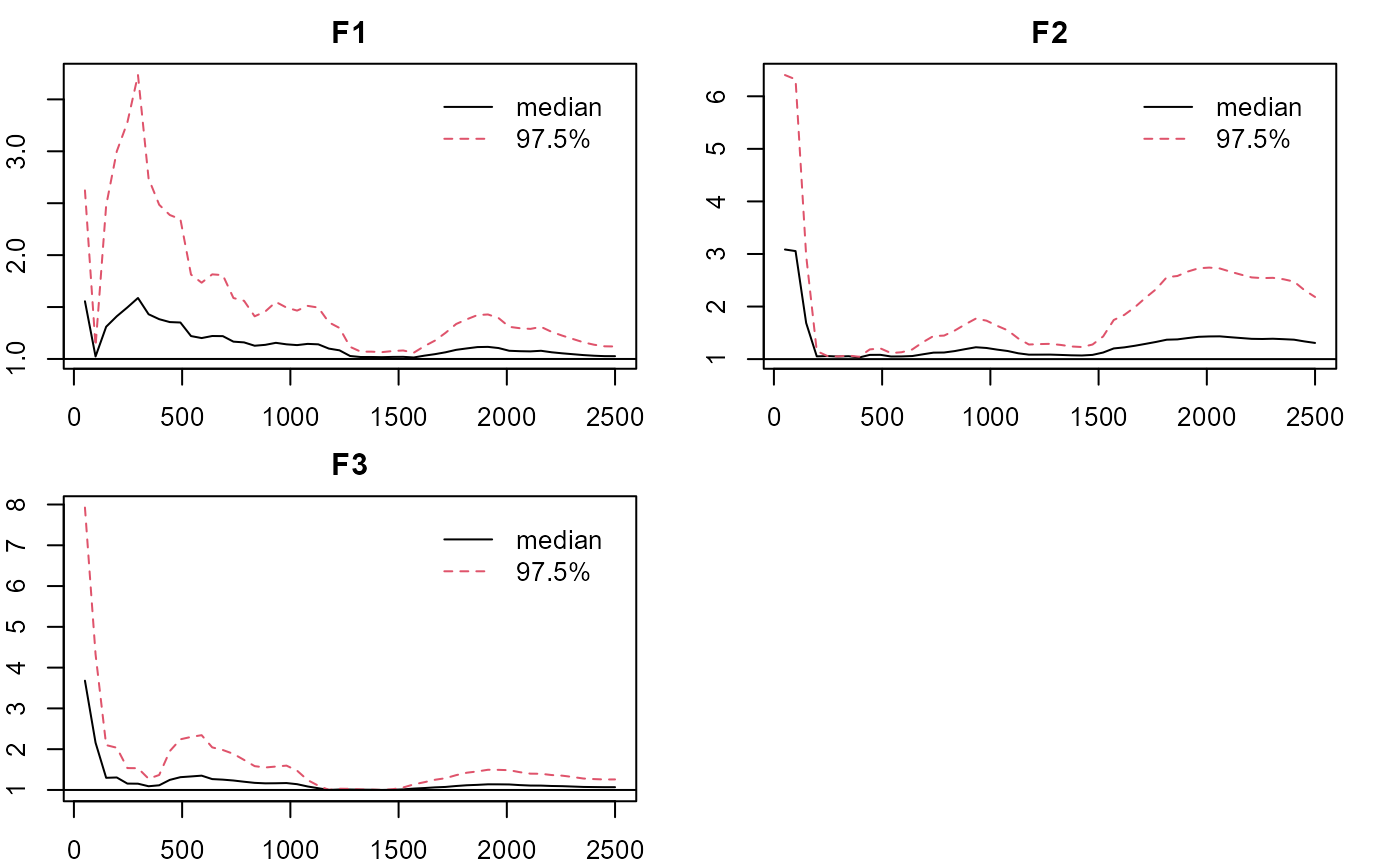
- C-step: Reconfigure the Q matrix for the C-step with one specified loading per item based on results from the E-step. Estimate with the PCFA model by setting LD=TRUE (by default). The estimates are more accurate, and the LD terms can be largely recovered.
Q<-matrix(-1,J,K);
tmp<-summary(m0, what="qlambda")
cind<-apply(tmp,1,which.max)
Q[cbind(c(1:J),cind)]<-1
Q
## [,1] [,2] [,3]
## [1,] 1 -1 -1
## [2,] 1 -1 -1
## [3,] 1 -1 -1
## [4,] 1 -1 -1
## [5,] 1 -1 -1
## [6,] 1 -1 -1
## [7,] -1 1 -1
## [8,] -1 1 -1
## [9,] -1 1 -1
## [10,] -1 1 -1
## [11,] -1 1 -1
## [12,] -1 1 -1
## [13,] -1 -1 1
## [14,] -1 -1 1
## [15,] -1 -1 1
## [16,] -1 -1 1
## [17,] -1 -1 1
## [18,] -1 -1 1## $NJK
## [1] 1000 18 3
##
## $`Miss%`
## [1] 0
##
## $`LD Allowed`
## [1] TRUE
##
## $`Burn in`
## [1] 5000
##
## $Iteration
## [1] 5000
##
## $`No. of sig lambda`
## [1] 22
##
## $Selected
## [1] TRUE TRUE TRUE
##
## $`Auto, NCONV, MCONV`
## [1] 0 0 10
##
## $EPSR
## Point est. Upper C.I.
## [1,] 1.0230 1.0636
## [2,] 1.0309 1.1124
## [3,] 1.2228 1.7416
##
## $`No. of sig LD terms`
## [1] 6
##
## $`DIC, BIC, AIC`
## [1] 3670.479 2706.037 1587.069
##
## $Time
## user system elapsed
## 92.36 0.00 92.46
summary(m1, what = 'qlambda')## 1 2 3
## I1 0.6915 0.0000 0.0000
## I2 0.6730 0.0000 0.0000
## I3 0.7588 0.0000 0.0000
## I4 0.7633 0.0000 0.0000
## I5 0.7623 0.0000 0.0000
## I6 0.7309 0.0000 0.0000
## I7 0.0000 0.7467 0.0000
## I8 0.0000 0.6745 0.0000
## I9 0.0000 0.7462 0.0000
## I10 0.0000 0.7270 0.0000
## I11 0.0000 0.7184 0.2125
## I12 0.0000 0.7324 0.2005
## I13 0.0000 0.0000 0.7128
## I14 0.0000 0.0000 0.6762
## I15 0.0000 0.0000 0.7225
## I16 0.0000 0.0000 0.7213
## I17 0.2542 0.0000 0.7095
## I18 0.2385 0.0000 0.7155
summary(m1,what='eigen')## est sd lower upper sig
## F1 3.4266 0.3704 2.7396 4.2256 1
## F2 3.3057 0.3302 2.6959 3.9784 1
## F3 3.2109 0.3410 2.6139 3.9488 1
summary(m1, what = 'offpsx')## row col est sd lower upper sig
## [1,] 14 1 0.2918 0.0479 0.1996 0.3825 1
## [2,] 7 2 0.2569 0.0480 0.1648 0.3496 1
## [3,] 4 3 0.2661 0.0683 0.1246 0.3898 1
## [4,] 13 8 0.2799 0.0451 0.1976 0.3783 1
## [5,] 10 9 0.2971 0.0665 0.1525 0.4270 1
## [6,] 16 15 0.2688 0.0704 0.1258 0.3978 1- CFA-LD: Configure the Q matrix for a CFA model with local dependence (i.e. without any unspecified loading) based on results from the C-step. Results are better than, but similar to the C-step.
Q<-summary(m1, what="qlambda")
Q[Q!=0]<-1
Q
## 1 2 3
## I1 1 0 0
## I2 1 0 0
## I3 1 0 0
## I4 1 0 0
## I5 1 0 0
## I6 1 0 0
## I7 0 1 0
## I8 0 1 0
## I9 0 1 0
## I10 0 1 0
## I11 0 1 1
## I12 0 1 1
## I13 0 0 1
## I14 0 0 1
## I15 0 0 1
## I16 0 0 1
## I17 1 0 1
## I18 1 0 1## $NJK
## [1] 1000 18 3
##
## $`Miss%`
## [1] 0
##
## $`LD Allowed`
## [1] TRUE
##
## $`Burn in`
## [1] 5000
##
## $Iteration
## [1] 5000
##
## $`No. of sig lambda`
## [1] 22
##
## $Selected
## [1] TRUE TRUE TRUE
##
## $`Auto, NCONV, MCONV`
## [1] 0 0 10
##
## $EPSR
## Point est. Upper C.I.
## [1,] 1.0222 1.1003
## [2,] 1.2677 1.9349
## [3,] 1.0009 1.0028
##
## $`No. of sig LD terms`
## [1] 26
##
## $`DIC, BIC, AIC`
## [1] 4851.891 3231.894 2269.974
##
## $Time
## user system elapsed
## 71.68 0.11 71.85
summary(m2, what = 'qlambda') ## 1 2 3
## I1 0.6514 0.0000 0.0000
## I2 0.6837 0.0000 0.0000
## I3 0.7026 0.0000 0.0000
## I4 0.6882 0.0000 0.0000
## I5 0.8461 0.0000 0.0000
## I6 0.8415 0.0000 0.0000
## I7 0.0000 0.6948 0.0000
## I8 0.0000 0.6235 0.0000
## I9 0.0000 0.6198 0.0000
## I10 0.0000 0.5916 0.0000
## I11 0.0000 0.6317 0.2934
## I12 0.0000 0.6082 0.2875
## I13 0.0000 0.0000 0.6595
## I14 0.0000 0.0000 0.6769
## I15 0.0000 0.0000 0.7223
## I16 0.0000 0.0000 0.7395
## I17 0.3054 0.0000 0.6916
## I18 0.2926 0.0000 0.6915
summary(m2,what='eigen')## est sd lower upper sig
## F1 3.4757 0.2171 3.0650 3.9089 1
## F2 2.3975 0.3131 1.7467 2.9940 1
## F3 3.1007 0.1769 2.7689 3.4376 1
summary(m2, what = 'offpsx')## row col est sd lower upper sig
## [1,] 7 1 -0.0726 0.0331 -0.1347 -0.0077 1
## [2,] 8 1 -0.0683 0.0333 -0.1305 -0.0017 1
## [3,] 9 1 -0.0845 0.0359 -0.1489 -0.0094 1
## [4,] 10 1 -0.0976 0.0357 -0.1624 -0.0233 1
## [5,] 11 1 -0.0753 0.0329 -0.1383 -0.0134 1
## [6,] 12 1 -0.0725 0.0333 -0.1328 -0.0027 1
## [7,] 14 1 0.2992 0.0305 0.2432 0.3603 1
## [8,] 7 2 0.2045 0.0408 0.1245 0.2854 1
## [9,] 11 2 -0.0881 0.0359 -0.1559 -0.0191 1
## [10,] 12 2 -0.0766 0.0375 -0.1481 -0.0010 1
## [11,] 4 3 0.3159 0.0581 0.1976 0.4252 1
## [12,] 7 3 -0.0869 0.0326 -0.1504 -0.0197 1
## [13,] 12 3 -0.0887 0.0327 -0.1529 -0.0245 1
## [14,] 7 4 -0.0791 0.0331 -0.1415 -0.0098 1
## [15,] 11 4 -0.0670 0.0322 -0.1345 -0.0072 1
## [16,] 12 4 -0.0810 0.0326 -0.1447 -0.0153 1
## [17,] 11 8 0.1067 0.0540 0.0110 0.2166 1
## [18,] 12 8 0.1216 0.0590 0.0158 0.2426 1
## [19,] 13 8 0.3333 0.0351 0.2669 0.4051 1
## [20,] 10 9 0.4249 0.0822 0.2734 0.6082 1
## [21,] 11 9 0.1080 0.0607 0.0114 0.2481 1
## [22,] 12 9 0.1357 0.0676 0.0128 0.2824 1
## [23,] 11 10 0.1071 0.0616 0.0057 0.2418 1
## [24,] 12 10 0.1239 0.0670 0.0055 0.2700 1
## [25,] 12 11 0.1200 0.0579 0.0206 0.2423 1
## [26,] 16 15 0.2403 0.0620 0.1137 0.3750 1