Note: the estimation process can be time consuming depending on the computing power. You can same some time by reducing the length of the chains.
Continuous Data w/o Local Dependence:
- Load the package, obtain the data, loading pattern (qlam), and setup the design matrix Q.
library(LAWBL)
dat <- sim18cfa0$dat
J <- ncol(dat) # no. of items
K <- 3 # no. of factors
qlam <- sim18cfa0$qlam
qlam
R>       [,1] [,2] [,3]
R>  [1,]  0.7  0.0  0.0
R>  [2,]  0.7  0.0  0.0
R>  [3,]  0.7  0.0  0.0
R>  [4,]  0.7  0.0  0.0
R>  [5,]  0.7  0.3  0.0
R>  [6,]  0.7  0.3  0.0
R>  [7,]  0.0  0.7  0.0
R>  [8,]  0.0  0.7  0.0
R>  [9,]  0.0  0.7  0.0
R> [10,]  0.0  0.7  0.0
R> [11,]  0.0  0.7  0.3
R> [12,]  0.0  0.7  0.3
R> [13,]  0.0  0.0  0.7
R> [14,]  0.0  0.0  0.7
R> [15,]  0.0  0.0  0.7
R> [16,]  0.0  0.0  0.7
R> [17,]  0.3  0.0  0.7
R> [18,]  0.3  0.0  0.7

Q<-matrix(-1,J,K); # -1 for unspecified items
Q[1:2,1]<-Q[7:8,2]<-Q[13:14,3]<-1 # 1 for specified items
Q
R>       [,1] [,2] [,3]
R>  [1,]    1   -1   -1
R>  [2,]    1   -1   -1
R>  [3,]   -1   -1   -1
R>  [4,]   -1   -1   -1
R>  [5,]   -1   -1   -1
R>  [6,]   -1   -1   -1
R>  [7,]   -1    1   -1
R>  [8,]   -1    1   -1
R>  [9,]   -1   -1   -1
R> [10,]   -1   -1   -1
R> [11,]   -1   -1   -1
R> [12,]   -1   -1   -1
R> [13,]   -1   -1    1
R> [14,]   -1   -1    1
R> [15,]   -1   -1   -1
R> [16,]   -1   -1   -1
R> [17,]   -1   -1   -1
R> [18,] -1 -1 -1- E-step: Estimate with the PCFA-LI model (E-step) by setting LD=F. Only a few loadings need to be specified in Q (e.g., 2 per factor). Longer chain is suggested for stabler performance (burn=iter=5,000 by default).
m0 <- pcfa(dat = dat, Q = Q,LD = FALSE, burn = 2000, iter = 2000,verbose = TRUE)
R>
R> Tot. Iter = 1000
R>          [,1]  [,2]  [,3]
R> Feigen  4.027 3.873 2.503
R> NLA_lg3 8.000 6.000 6.000
R> Shrink  3.219 3.219 3.219
R>
R> Tot. Iter = 2000
R>          [,1]  [,2]  [,3]
R> Feigen  3.626 3.688 4.227
R> NLA_lg3 6.000 6.000 6.000
R> Shrink  2.705 2.705 2.705
R>
R> Tot. Iter = 3000
R>          [,1]  [,2]  [,3]
R> Feigen  3.757 3.545 4.346
R> NLA_lg3 6.000 6.000 7.000
R> Shrink  3.614 3.614 3.614
R> Adj PSR 1.092 1.809 1.729
R>
R> Tot. Iter = 4000
R>          [,1]  [,2]  [,3]
R> Feigen  2.677 3.699 3.423
R> NLA_lg3 6.000 6.000 7.000
R> Shrink  3.153 3.153 3.153
R> Adj PSR 1.001 1.006 1.021
R>
R> #Sign change: 0 0 0 0 0 0
R>    user  system elapsed
R>   16.53    0.02   16.56

# summarize basic information
summary(m0)
R> $N
R> [1] 1000
R>
R> $J
R> [1] 18
R>
R> $K
R> [1] 3
R>
R> $`Miss%`
R> [1] 0
R>
R> $`LD enabled`
R> [1] FALSE
R>
R> $`Burn in`
R> [1] 2000
R>
R> $Iteration
R> [1] 2000
R>
R> $`No. of sig lambda`
R> [1] 24
R>
R> $`Adj. PSR`
R>    Point est. Upper C.I.
R> F1   1.000692   1.000992
R> F2   1.006334   1.030777
R> F3   1.020804   1.022674

#summarize significant loadings in pattern/Q-matrix format
summary(m0, what = 'qlambda')
R>          [,1]      [,2]      [,3]
R> I1  0.6881938 0.0000000 0.0000000
R> I2  0.7276617 0.0000000 0.0000000
R> I3  0.7053776 0.0000000 0.0000000
R> I4  0.6525335 0.0000000 0.0000000
R> I5  0.7120300 0.2865062 0.0000000
R> I6  0.7095454 0.2982842 0.0000000
R> I7  0.0000000 0.7413281 0.0000000
R> I8  0.0000000 0.7388007 0.0000000
R> I9  0.0000000 0.7328911 0.0000000
R> I10 0.0000000 0.6653911 0.0000000
R> I11 0.0000000 0.7037540 0.2547656
R> I12 0.0000000 0.7147327 0.2628362
R> I13 0.0000000 0.0000000 0.7521188
R> I14 0.0000000 0.0000000 0.7831557
R> I15 0.0000000 0.0000000 0.7695287
R> I16 0.0000000 0.0000000 0.7263737
R> I17 0.2407217 0.0000000 0.7269717
R> I18 0.2450948 0.0000000 0.7290218

#factorial eigenvalue
summary(m0,what='eigen')
R>         est        sd    lower    upper sig
R> F1 3.157885 0.5277766 2.128743 4.166953   1
R> F2 3.387151 0.4077793 2.640005 4.243836   1
R> F3 3.600655 0.4920634 2.666980 4.561343   1

#plotting factorial eigenvalue
plot_eigen(m0) # trace
plot_eigen(m0, what='density') #density

plot_eigen(m0, what='APSR') #adj, PSRF
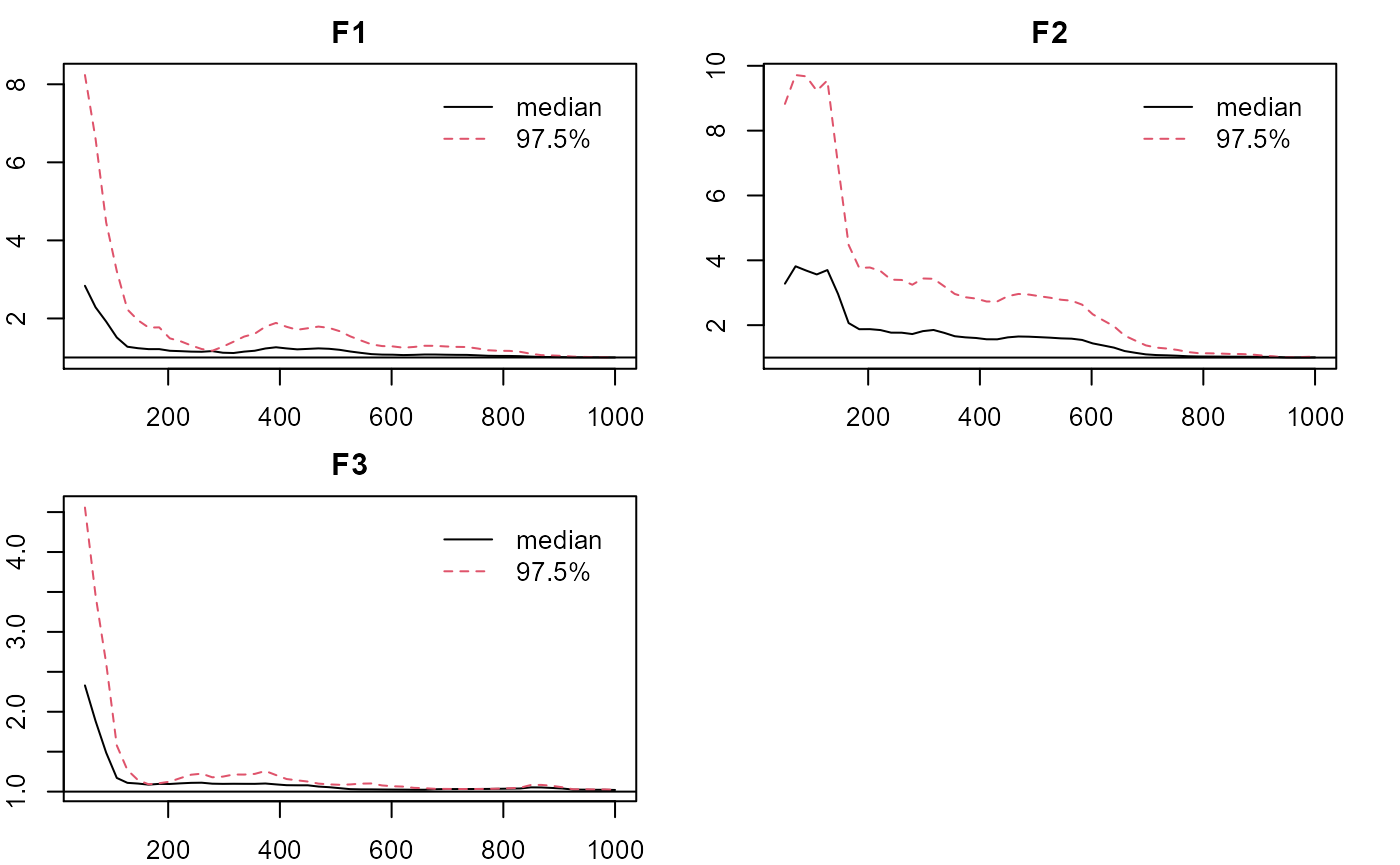
- C-step: Reconfigure the Q matrix for the C-step with one specified loading per item based on results from the E-step. Estimate with the PCFA model by setting LD=TRUE (by default). Longer chain is suggested for stabler performance. Results are very close to the E-step, since there’s no LD in the data.
Q<-matrix(-1,J,K);
tmp<-summary(m0, what="qlambda")
cind<-apply(tmp,1,which.max)
Q[cbind(c(1:J),cind)]<-1
#alternatively
#Q[1:6,1]<-Q[7:12,2]<-Q[13:18,3]<-1 # 1 for specified items

m1 <- pcfa(dat = dat, Q = Q, burn = 2000, iter = 2000,verbose = TRUE)
summary(m1)
summary(m1, what = 'qlambda')
summary(m1, what = 'offpsx') #summarize significant LD terms
summary(m1,what='eigen')

#plotting factorial eigenvalue
# par(mar = rep(2, 4))
plot_eigen(m1) # trace
plot_eigen(m1, what='density') #density
plot_eigen(m1, what='APSR') #adj, PSRF
- CFA-LD: One can also configure the Q matrix for a CFA model with local dependence (i.e. without any unspecified loading) based on results from the C-step. Results are also very close.
Continuous Data with Local Dependence:
- Load the the data, loading pattern (qlam), and LD terms, and setup the design matrix Q.
dat <- sim18cfa1$dat
J <- ncol(dat) # no. of items
K <- 3 # no. of factors
sim18cfa1$qlam
sim18cfa1$LD # effect size = .3

Q<-matrix(-1,J,K); # -1 for unspecified items
Q[1:2,1]<-Q[7:8,2]<-Q[13:14,3]<-1 # 1 for specified items
Q
- E-step: Estimate with the PCFA-LI model (E-step) by setting LD=FALSE. Only a few loadings need to be specified in Q (e.g., 2 per factor). Some loading estimates are biased due to ignoring the LD. So do the eigenvalues.
m0 <- pcfa(dat = dat, Q = Q,LD = FALSE, burn = 4000, iter = 4000,verbose = TRUE)
summary(m0)
summary(m0, what = 'qlambda')
summary(m0,what='eigen')

plot_eigen(m0) # trace
plot_eigen(m0, what='APSR')
- C-step: Reconfigure the Q matrix for the C-step with one specified loading per item based on results from the E-step. Estimate with the PCFA model by setting LD=TRUE (by default). The estimates are more accurate, and the LD terms can be largely recovered.
Q<-matrix(-1,J,K);
tmp<-summary(m0, what="qlambda")
cind<-apply(tmp,1,which.max)
Q[cbind(c(1:J),cind)]<-1
Q

m1 <- pcfa(dat = dat, Q = Q,burn = 4000, iter = 4000,verbose = TRUE)
summary(m1)
summary(m1, what = 'qlambda')
summary(m1,what='eigen')
summary(m1, what = 'offpsx')
- CFA-LD: Configure the Q matrix for a CFA model with local dependence (i.e. without any unspecified loading) based on results from the C-step. Results are better than, but similar to the C-step.